exportgraphics
Save plot or graphics content to file
Description
exportgraphics(
saves the contents of the graphics object specified by obj,filename)obj to a file. The
graphics object can be any type of axes, a figure, a standalone visualization, a tiled chart
layout, or a container within the figure. The resulting graphic is tightly cropped to a thin
margin surrounding your content.
exportgraphics(
specifies additional options for saving the file. For example,
obj,filename,Name,Value)exportgraphics(gca,'myplot.jpg','Resolution',300) saves the contents of
the current axes as a 300-DPI image file.
Examples
Export Axes as Image File
Create a line plot and get the current axes. Then save the contents of the axes as a JPEG file.
plot(rand(5,5))
ax = gca;
exportgraphics(ax,'LinePlot.jpg')
Specify Image Resolution
Display an image and get the current axes. Then save the contents of the axes as a 300-DPI JPEG file.
I = imread('peppers.png');
imshow(I)
ax = gca;
exportgraphics(ax,'Peppers300.jpg','Resolution',300)

Export Figure
Display a plot with an annotation that extends beyond the bounds of the axes. Save the contents of the figure as a PDF file.
plot(1:10)
annotation('textarrow',[0.06 0.5],[0.73 0.5],'String','y = x ')
f = gcf;
exportgraphics(f,'AnnotatedPlot.pdf')

Export as PDF Containing Only Vector Graphics
Display a bar chart and get the current axes. Then save the contents of the axes as a PDF containing only vector graphics.
bar([10 22 31 43])
ax = gca;
exportgraphics(ax,'BarChart.pdf','ContentType','vector')

Export Tiled Chart Layout
Display two plots in a tiled chart layout. Then save both plots as a PDF by passing the TiledChartLayout object to the exportgraphics function.
t = tiledlayout(2,1);
nexttile
plot([1 2 3])
nexttile
plot([3 2 1])
exportgraphics(t,'Layout.pdf')
If you want to save just one of the plots in the layout, call the nexttile function with the axes return argument. Then pass the axes to the exportgraphics function.
Export Heatmap as PDF With Transparent Background
Display a heatmap chart. Then save the chart as a PDF containing only vector graphics with a transparent background.
h = heatmap(rand(10,10));
exportgraphics(h,'Hmap.pdf','BackgroundColor','none','ContentType','vector')

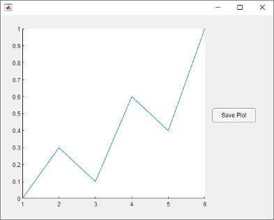
Create App for Saving Plot
Create a program file called saveapp.m that displays a plot and a
button for saving the axes content. In the callback function for the button, call the
uiputfile function to prompt the user for a file name and location.
Then call the exportgraphics function with the full path to the
specified file.
function saveapp
f = uifigure;
ax = uiaxes(f,'Position',[25 25 400 375]);
plot(ax,[0 0.3 0.1 0.6 0.4 1])
b = uibutton(f,'Position',[435 200 90 30],'Text','Save Plot');
b.ButtonPushedFcn = @buttoncallback;

    function buttoncallback(~,~)
        filter = {'*.jpg';'*.png';'*.tif';'*.pdf';'*.eps'};
        [filename,filepath] = uiputfile(filter);
        if ischar(filename)
            exportgraphics(ax,[filepath filename]);
        end
    end
end
Run the app by calling the saveapp function. When you click the
Save Plot button in the app, a dialog box prompts you for a
file name and location. Then the axes content is saved in the specified file. The area
surrounding the axes, including the button, is not included in the file.
saveapp
Input Arguments
obj — Graphics object
axes | figure | standalone visualization | tiled chart layout | ...
Graphics object, specified as one of these objects:
Any type of axes: an
Axes,PolarAxes, orGeographicAxesobject.A figure created with either the
figureoruifigurefunction.A standalone visualization such a
heatmapchart.A tiled chart layout, which you create with the
tiledlayoutfunction.A container within a figure: a
Panel,Tab, orButtonGroupobject.
Capture Area
exportgraphics captures the contents of the object you
specify. It does not capture UI components such as buttons or sliders.
It also does not capture adjacent containers or child containers. For example, consider a figure containing a line plot with an adjacent panel containing a heatmap:
f = figure;
ax = axes(f,'Position',[0.1 0.1 0.4 0.8]);
plot(ax,[0 1])
p = uipanel(f,'Position',[0.55 0.1 0.4 0.8]);
heatmap(p,rand(10,5))

exportgraphics(f,'myfigure.png')
exportgraphics(p,'mypanel.png')

When you run the preceding code, myfigure.png contains the line
plot, but not the heatmap. Similarly, mypanel.png contains the
heatmap, but not the line plot.
filename — File name
character vector | string scalar
File name, specified as a character vector or a string scalar that includes the file
extension. If filename does not include a full path, MATLAB® saves the file in the current folder. You must have permission to write to
the file.
The following table lists the supported file formats and the file extensions (which are not case sensitive).
| File Format | File Extension |
|---|---|
Joint Photographic Experts Group (JPEG) | 'jpg' or 'jpeg' |
Portable Network Graphics (PNG) | 'png' |
Tagged Image File Format (TIFF) | 'tif' or 'tiff' |
Portable Document Format (PDF) The PDF includes
embeddable fonts when the | 'pdf' |
Enhanced Metafile for Windows® systems only (EMF) | 'emf' |
Encapsulated PostScript® (EPS) | 'eps' |
Example: exportgraphics(gca,'myfile.jpg') saves the contents of
the current axes to a JPEG file called myfile.jpg.
Name-Value Pair Arguments
Specify optional
comma-separated pairs of Name,Value arguments. Name is
the argument name and Value is the corresponding value.
Name must appear inside quotes. You can specify several name and value
pair arguments in any order as
Name1,Value1,...,NameN,ValueN.
exportgraphics(gca,'myplot.jpg','Resolution',300) saves the
contents of the current axes to a 300-DPI image file.'BackgroundColor' — Background color
[1 1 1] (default) | 'current' | 'none' | RGB triplet | 'r' | 'g' | 'b' | ...
Background color, specified as 'current',
'none', an RGB triplet, a hexadecimal color code, or a color
name. The background color controls the color of the margin that surrounds the axes or chart.
A value of
'current'sets the background color to the parent container's color.A value of
'none'sets the background color to transparent or white, depending on the file format and the value ofContentType:Transparent — For files with
ContentType='vector'White — For image files, or when
ContentType='image'When
ContentType='auto', MATLAB sets the background color according to the heuristic it uses to determine the type content to save.
Alternatively, specify a custom color or a named color.
Custom Colors and Named Colors
RGB triplets and hexadecimal color codes are useful for specifying custom colors.
An RGB triplet is a three-element row vector whose elements specify the intensities of the red, green, and blue components of the color. The intensities must be in the range
[0,1]; for example,[0.4 0.6 0.7].A hexadecimal color code is a character vector or a string scalar that starts with a hash symbol (
#) followed by three or six hexadecimal digits, which can range from0toF. The values are not case sensitive. Thus, the color codes'#FF8800','#ff8800','#F80', and'#f80'are equivalent.
Alternatively, you can specify some common colors by name. This table lists the named color options, the equivalent RGB triplets, and hexadecimal color codes.
| Color Name | Short Name | RGB Triplet | Hexadecimal Color Code | Appearance |
|---|---|---|---|---|
'red' | 'r' | [1 0 0] | '#FF0000' |
|
'green' | 'g' | [0 1 0] | '#00FF00' |
|
'blue' | 'b' | [0 0 1] | '#0000FF' |
|
'cyan' | 'c' | [0 1 1] | '#00FFFF' |
|
'magenta' | 'm' | [1 0 1] | '#FF00FF' |
|
'yellow' | 'y' | [1 1 0] | '#FFFF00' |
|
'black' | 'k' | [0 0 0] | '#000000' |
|
'white' | 'w' | [1 1 1] | '#FFFFFF' |
|
Here are the RGB triplets and hexadecimal color codes for the default colors MATLAB uses in many types of plots.
| RGB Triplet | Hexadecimal Color Code | Appearance |
|---|---|---|
[0 0.4470 0.7410] | '#0072BD' |
|
[0.8500 0.3250 0.0980] | '#D95319' |
|
[0.9290 0.6940 0.1250] | '#EDB120' |
|
[0.4940 0.1840 0.5560] | '#7E2F8E' |
|
[0.4660 0.6740 0.1880] | '#77AC30' |
|
[0.3010 0.7450 0.9330] | '#4DBEEE' |
|
[0.6350 0.0780 0.1840] | '#A2142F' |
|
Alternative Functionality
Hovering over the Export button ![]() in the axes toolbar reveals a drop-down menu with options for
exporting content:
in the axes toolbar reveals a drop-down menu with options for
exporting content:
 : Save the content as a tightly cropped image or
PDF.
: Save the content as a tightly cropped image or
PDF. : Copy the content as an image.
 : Copy the content as a vector graphic.