Configure Array Plot Block
Signal Display
The following figure highlights the important aspects of the Array Plot window.

Minimum x-axis limit — Array Plot sets the minimum x-axis limit using the value of the X-offset property. To change the X-offset, select View > Configuration Properties. In the Configuration Properties, on the Main tab, modify the X-offset.
Maximum x-axis limit — Array Plot sets the maximum x-axis limit by summing the value of X-offset parameter with the span of x-axis values. The relationship between the span of the x-axis data to the
SampleIncrementproperty is determined by this equation:If you set
SampleIncrementto0.1and the input signal data has 51 samples. The scope displays values on the x-axis from0to5. If you also set the X-offset to–2.5, the scope displays values on the x-axis from–2.5to2.5. The values on the x-axis of the scope display remain the same throughout simulation.Status — Provides the current status of the plot. The status can be either of the following conditions:
Processing— Occurs after you run the model and before the simulation ends.Stopped— Occurs after you construct the scope object and before you run the simulation. This status also occurs after the simulation ends.
Multiple Signal Names and Colors
By default, if the input signal has multiple channels, the scope uses an index
number to identify each channel of that signal. For example, a 2-channel signal
would have the following default names in the channel legend: Channel
1, Channel 2. To show the legend, select View > Configuration Properties, click the Display tab, and select the
Show Legend check box. If there are a total of seven input
channels, the following legend appears in the display.

By default, the scope has a black axes background and chooses line colors for each channel in a manner similar to the Simulink® Scope (Simulink) block. When the scope axes background is black, it assigns each channel of each input signal a line color in the order shown in the above figure.
If there are more than seven channels, then the scope repeats this order to assign
line colors to the remaining channels. To choose line colors for each channel,
change the axes background color to any color except black. To change the axes
background color to white, select View > Style, click the Axes background color button (![]() ), and select white from the color palette. Run
the simulation again. The following legend appears in the display. This image shows
the color order when the background is not black.
), and select white from the color palette. Run
the simulation again. The following legend appears in the display. This image shows
the color order when the background is not black.

Array Plot Measurement Panels
The Measurements panels are the panels that appear to the right side of the Array Plot figure. These panels are labeled Trace selection, Cursor Measurements, Signal Statistics, and Peak Finder.
Trace Selection Panel
When you use the scope to view multiple signals, the Trace Selection panel appears. Use this panel to select which signal to measure. To open the Trace Selection panel:
From the menu, select Tools > Measurements > Trace Selection.
Open a measurement panel.
-

Cursor Measurements Panel
The Cursor Measurements panel displays screen cursors. The panel provides two types of cursors for measuring signals. Waveform cursors are vertical cursors that track along the signal. Screen cursors are both horizontal and vertical cursors that you can place anywhere in the display.
Note
If a data point in your signal has more than one value, the cursor measurement at that point is undefined and no cursor value is displayed.
Display screen cursors with signal times and values. To open the Cursor measurements panel:
From the menu, select Tools > Measurements > Cursor Measurements.
On the toolbar, click the Cursor Measurements
 button.
In the Settings pane, you can modify the type of screen cursors used for calculating measurements. When more than one signal is displayed, you can assign cursors to each trace individually.

Screen Cursors — Shows screen cursors (for spectrum and dual view only).
Horizontal — Shows horizontal screen cursors (for spectrum and dual view only).
Vertical — Shows vertical screen cursors (for spectrum and dual view only).
Waveform Cursors — Shows cursors that attach to the input signals (for spectrum and dual view only).
Lock Cursor Spacing — Locks the frequency difference between the two cursors.
Snap to Data — Positions the cursors on signal data points.
The Measurements pane displays time and value measurements.

1 — View or modify the time or value at cursor number one (solid line cursor).
2 — View or modify the time or value at cursor number two (dashed line cursor).
ΔT or ΔX — Shows the absolute value of the time (x-axis) difference between cursor number one and cursor number two.
ΔY — Shows the absolute value of the signal amplitude difference between cursor number one and cursor number two.
1/ΔT or 1/ΔX — Shows the rate. The reciprocal of the absolute value of the difference in the times (x-axis) between cursor number one and cursor number two.
ΔY/ΔT or ΔY/ΔX — Shows the slope. The ratio of the absolute value of the difference in signal amplitudes between cursors to the absolute value of the difference in the times (x-axis) between cursors.
Signal Statistics Panel
Display signal statistics for the signal selected in the Trace Selection panel. To open the Signal Statistics panel:
From the menu, select Tools > Measurements > Signal Statistics.
On the toolbar, click the Signal Statistics
 button.

The statistics shown are:
Max — Maximum or largest value within the displayed portion of the input signal.
Min — Minimum or smallest value within the displayed portion of the input signal.
Peak to Peak — Difference between the maximum and minimum values within the displayed portion of the input signal.
Mean — Average or mean of all the values within the displayed portion of the input signal.
Median — Median value within the displayed portion of the input signal.
RMS — Root mean squared of the input signal.
When you use the zoom options in the scope, the Signal Statistics measurements automatically adjust to the time range shown in the display. In the scope toolbar, click the Zoom In or Zoom X button to constrict the x-axis range of the display, and the statistics shown reflect this time range. For example, you can zoom in on one pulse to make the Signal Statistics panel display information about only that particular pulse.
The Signal Statistics measurements are valid for any units of the input signal. The letter after the value associated with each measurement represents the appropriate International System of Units (SI) prefix, such as m for milli-. For example, if the input signal is measured in volts, an m next to a measurement value indicates that this value is in units of millivolts.
Peak Finder Panel
The Peak Finder panel displays the maxima, showing the x-axis values at which they occur. Peaks are defined as a local maximum where lower values are present on both sides of a peak. Endpoints are not considered peaks. This panel allows you to modify the settings for peak threshold, maximum number of peaks, and peak excursion.
From the menu, select Tools > Measurements > Peak Finder.
On the toolbar, click the Peak Finder
 button.
The Settings pane enables you to modify the parameters used to calculate the peak values within the
displayed portion of the input signal. For more information on the algorithms this pane uses, see the findpeaks function reference.

Properties to set:
Peak Threshold — The level above which peaks are detected. This setting is equivalent to the
MINPEAKHEIGHTparameter, which you can set when you run thefindpeaksfunction.Max Num of Peaks — The maximum number of peaks to show. The value you enter must be a scalar integer from 1 through 99. This setting is equivalent to the
NPEAKSparameter, which you can set when you run thefindpeaksfunction.Min Peaks Distance — The minimum number of samples between adjacent peaks. This setting is equivalent to the
MINPEAKDISTANCEparameter, which you can set when you run thefindpeaksfunction.Peak Excursion — The minimum height difference between a peak and its neighboring samples. Peak excursion is illustrated alongside peak threshold in the following figure.

The peak threshold is a minimum value necessary for a sample value to be a peak. The peak excursion is the minimum difference between a peak sample and the samples to its left and right in the time domain. In the figure, the green vertical line illustrates the lesser of the two height differences between the labeled peak and its neighboring samples. This height difference must be greater than the Peak Excursion value for the labeled peak to be classified as a peak. Compare this setting to peak threshold, which is illustrated by the red horizontal line. The amplitude must be above this horizontal line for the labeled peak to be classified as a peak.
The peak excursion setting is equivalent to the
THRESHOLDparameter, which you can set when you run thefindpeaksfunction.Label Format — The coordinates to display next to the calculated peak values on the plot. To see peak values, you must first expand the Peaks pane and select the check boxes associated with individual peaks of interest. By default, both x-axis and y-axis values are displayed on the plot. Select which axes values you want to display next to each peak symbol on the display.
X+Y— Display both x-axis and y-axis values.X— Display only x-axis values.Y— Display only y-axis values.
The Peaks pane displays the largest calculated peak values. It also shows the coordinates at which the peaks occur, using the parameters you define in the Settings pane. You set the Max Num of Peaks parameter to specify the number of peaks shown in the list.
The numerical values displayed in the Value column are equivalent to the pks
output argument returned when you run the findpeaks function. The numerical values displayed in the
second column are similar to the locs output argument returned when you run the
findpeaks function.
The Peak Finder displays the peak values in the Peaks pane. By default, the Peak Finder panel displays the largest calculated peak values in the Peaks pane in decreasing order of peak height.
Use the check boxes to control which peak values are shown on the display. By default, all check boxes are cleared and the Peak Finder panel hides all the peak values. To show or hide all the peak values on the display, use the check box in the top-left corner of the Peaks pane.
The Peaks are valid for any units of the input signal. The letter after the value associated with each measurement indicates the abbreviation for the appropriate International System of Units (SI) prefix, such as m for milli-. For example, if the input signal is measured in volts, an m next to a measurement value indicates that this value is in units of millivolts.
Configuration Properties
The Configuration Properties dialog box controls various properties about the Array Plot display. From the Array Plot menu, select View > Configuration Properties to open this dialog box.
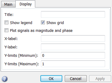

For more details about the properties, see Configuration Properties.
Style Dialog Box
In the Style dialog box, you can customize the style of displays. You are able to change the color of the figure containing the displays, the background and foreground colors of display axes, and properties of lines in a display. From the scope menu, select View > Style to open this dialog box.

For more details about the properties, see Style.
Axes Scaling Properties
The Tools—Plot Navigation Properties dialog box allows you to automatically zoom in on and zoom out of your data. You can also scale the axes of the scope. In the scope menu, select Tools > Axes Scaling > Axes Scaling Properties to open this dialog box.
For more details about the properties, see Axes Scaling Properties.