Buffering and Frame-Based Processing

Buffer Input into Frames

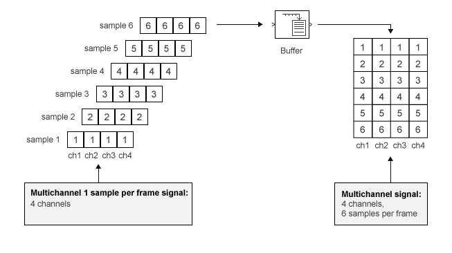
Multichannel signals of frame size 1 can be buffered into multichannel signals of frame size L using the Buffer block. L is greater than 1.

The following figure is a graphical representation of a signal with frame size 1 being converted into a signal of frame size L by the Buffer block.

In the following example, a two-channel 1 sample per frame signal is buffered into a two-channel 4 samples per frame signal using a Buffer block:

At the MATLAB^® command prompt, type ex_buffer_tut.
The Buffer Example model opens.
Double-click the Signal From Workspace block. The Source Block Parameters: Signal From Workspace dialog box opens.
Set the parameters as follows:
- Signal = [1:10;-1:-1:-10]'
- Sample time = 1
- Samples per frame = 1
- Form output after final data value = Setting to zero
Based on these parameters, the Signal from Workspace block outputs a signal with a frame length of 1 and a sample period of 1 second. Because you set the Samples per frame parameter setting to 1, the Signal From Workspace block outputs one two-channel sample at each sample time.
Save these parameters and close the dialog box by clicking OK.
Double-click the Buffer block. The Function Block Parameters: Buffer dialog box opens.
Set the parameters as follows:
- Output buffer size (per channel) = 4
- Buffer overlap = 0
- Initial conditions = 0
Because you set the Output buffer size parameter to 4, the Buffer block outputs a frame signal with frame size 4.
Run the model.
The figure below is a graphical interpretation of the model behavior during simulation.

Note

Alternatively, you can set the Samples per frame parameter of the Signal From Workspace block to 4 and create the same signal shown above without using a Buffer block. The Signal From Workspace block performs the buffering internally, in order to output a two-channel frame.

Buffer Signals into Frames with Overlap

In some cases it is useful to work with data that represents overlapping sections of an original signal. For example, in estimating the power spectrum of a signal, it is often desirable to compute the FFT of overlapping sections of data. Overlapping buffers are also needed in computing statistics on a sliding window, or for adaptive filtering.

The Buffer overlap parameter of the Buffer block specifies the number of overlap points, L. In the overlap case (L > 0), the frame period for the output is (M_o-L)*T_si, where T_si is the input sample period and M_o is the Buffer size.

Note

Set the Buffer overlap parameter to a negative value to achieve output frame rates slower than in the nonoverlapping case. The output frame period is still T_si*(M_o-L), but now with L < 0. Only the M_o newest inputs are included in the output buffers. The previous L inputs are discarded.

In the following example, a four-channel signal with frame length 1 and sample period 1 is buffered to a signal with frame size 3 and frame period 2. Because of the buffer overlap, the input sample period is not conserved, and the output sample period is 2/3:

At the MATLAB command prompt, type ex_buffer_tut3.
The Buffer Example T3 model opens.
Also, the variable sp_examples_src is loaded into the MATLAB workspace. This variable is defined as follows:
```
sp_examples_src=[1 1 5 -1; 2 1 5 -2; 3 0 5 -3; 4 0 5 -4; 5 1 5 -5; 6 1 5 -6];
```
Double-click the Signal From Workspace block. The Source Block Parameters: Signal From Workspace dialog box opens.
Set the block parameters as follows:
- Signal = sp_examples_src
- Sample time = 1
- Samples per frame = 1
- Form output after final data value by = Setting to zero
Based on these parameters, the Signal from Workspace block outputs a signal with a sample period of 1 second. Because you set the Samples per frame parameter setting to 1, the Signal From Workspace block outputs one four-channel sample at each sample time.
Save these parameters and close the dialog box by clicking OK.
Double-click the Buffer block. The Function Block Parameters: Buffer dialog box opens.
Set the block parameters as follows, and then click OK:
- Output buffer size (per channel) = 3
- Buffer overlap = 1
- Initial conditions = 0
Because you set the Output buffer size parameter to 3, the Buffer block outputs a signal with frame size 3. Also, because you set the Buffer overlap parameter to 1, the last sample from the previous output frame is the first sample in the next output frame.
Run the model.
The following figure is a graphical interpretation of the model's behavior during simulation.

At the MATLAB command prompt, type sp_examples_yout.

The following is displayed in the MATLAB Command Window.

sp_examples_yout =

     0     0     0     0
     0     0     0     0
     0     0     0     0
     0     0     0     0
     1     1     5    -1
     2     1     5    -2
     2     1     5    -2
     3     0     5    -3
     4     0     5    -4
     4     0     5    -4
     5     1     5    -5
     6     1     5    -6
     6     1     5    -6
     0     0     0     0
     0     0     0     0
     0     0     0     0
     0     0     0     0
     0     0     0     0

Notice that the inputs do not begin appearing at the output until the fifth row, the second row of the second frame. This is due to the block's latency.

See Excess Algorithmic Delay (Tasking Latency) for general information about algorithmic delay. For instructions on how to calculate buffering delay, see Buffer Delay and Initial Conditions.

Buffer Frame Inputs into Other Frame Inputs

In the following example, a two-channel signal with frame size 4 is rebuffered to a signal with frame size 3 and frame period 2. Because of the overlap, the input sample period is not conserved, and the output sample period is 2/3:

At the MATLAB command prompt, type ex_buffer_tut4.
The Buffer Example T4 model opens.
Also, the variable sp_examples_src is loaded into the MATLAB workspace. This variable is defined as
```
sp_examples_src = [1 1; 2 1; 3 0; 4 0; 5 1; 6 1; 7 0; 8 0]
```
Double-click the Signal From Workspace block. The Source Block Parameters: Signal From Workspace dialog box opens.
Set the block parameters as follows:
- Signal = sp_examples_src
- Sample time = 1
- Samples per frame = 4
Based on these parameters, the Signal From Workspace block outputs a two-channel frame signal with a sample period of 1 second and a frame size of 4.
Save these parameters and close the dialog box by clicking OK.
Double-click the Buffer block. The Function Block Parameters: Buffer dialog box opens.
Set the block parameters as follows, and then click OK:
- Output buffer size (per channel) = 3
- Buffer overlap = 1
- Initial conditions = 0
Based on these parameters, the Buffer block outputs a two-channel frame signal with a frame size of 3.
Run the model.
The following figure is a graphical representation of the model's behavior during simulation.
Note that the inputs do not begin appearing at the output until the last row of the third output matrix. This is due to the block's latency.

See Excess Algorithmic Delay (Tasking Latency) for general information about algorithmic delay. For instructions on how to calculate buffering delay, and see Buffer Delay and Initial Conditions.

Buffer Delay and Initial Conditions

In the examples Buffer Signals into Frames with Overlap and Buffer Frame Inputs into Other Frame Inputs, the input signal is delayed by a certain number of samples. The initial output samples correspond to the value specified for the Initial condition parameter. The initial condition is zero in both examples mentioned above.

Under most conditions, the Buffer and Unbuffer blocks have some amount of delay or latency. This latency depends on both the block parameter settings and the Simulink^® tasking mode. You can use the rebuffer_delay function to determine the length of the block's latency for any combination of frame size and overlap.

The syntax rebuffer_delay(f,n,v) returns the delay, in samples, introduced by the buffering and unbuffering blocks during multitasking operations, where f is the input frame size, n is the Output buffer size parameter setting, and v is the Buffer overlap parameter setting.

For example, you can calculate the delay for the model discussed in the Buffer Frame Inputs into Other Frame Inputs using the following command at the MATLAB command line:

d = rebuffer_delay(4,3,1)
d = 8

This result agrees with the block's output in that example. Notice that this model was simulated in Simulink multitasking mode.

For more information about delay, see Excess Algorithmic Delay (Tasking Latency). For delay information about a specific block, see the “Latency” section of the block reference page. For more information about the rebuffer_delay function, see rebuffer_delay.

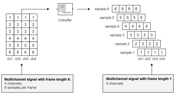
Unbuffer Frame Signals into Sample Signals

You can unbuffer multichannel signals of frame length greater than 1 into multichannel signals of frame length equal to 1 using the Unbuffer block. The Unbuffer block performs the inverse operation of the Buffer block's buffering process, where signals with frame length 1 are buffered into a signal with frame length greater than 1. The Unbuffer block generates an N-channel output containing one sample per frame from an N-channel input containing multiple channels per frame. The first row in each input matrix is always the first output.

The following figure is a graphical representation of this process.

The sample period of the output, T_so, is related to the input frame period, T_fi, by the input frame size, M_i.

$T_{s o} = T_{f i} / M_{i}$

The Unbuffer block always preserves the signal's sample period (T_so = T_si). See Convert Sample and Frame Rates in Simulink for more information about rate conversions.

In the following example, a two-channel signal with four samples per frame is unbuffered into a two-channel signal with one sample per frame:

At the MATLAB command prompt, type ex_unbuffer_tut.
The Unbuffer Example model opens.
Double-click the Signal From Workspace block. The Source Block Parameters: Signal From Workspace dialog box opens.
Set the block parameters as follows:
- Signal = [1:10;-1:-1:-10]'
- Sample time = 1
- Samples per frame = 4
- Form output after final data value by = Setting to zero
Based on these parameters, the Signal From Workspace block outputs a two-channel signal with frame size 4.
Save these parameters and close the dialog box by clicking OK.
Double-click the Unbuffer block. The Function Block Parameters: Unbuffer dialog box opens.
Set the Initial conditions parameter to 0, and then click OK.
The Unbuffer block unbuffers a two-channel signal with four samples per frame into a two-channel signal with one sample per frame.
Run the model.
The following figures is a graphical representation of what happens during the model simulation.
Note
The Unbuffer block generates initial conditions not shown in the figure below with the value specified by the Initial conditions parameter. See the Unbuffer reference page for information about the number of initial conditions that appear in the output.

At the MATLAB command prompt, type sp_examples_yout.

The following is a portion of the output.

sp_examples_yout(:,:,1) =

     0     0


sp_examples_yout(:,:,2) =

     0     0


sp_examples_yout(:,:,3) =

     0     0


sp_examples_yout(:,:,4) =

     0     0


sp_examples_yout(:,:,5) =

     1    -1


sp_examples_yout(:,:,6) =

     2    -2


sp_examples_yout(:,:,7) =

     3    -3

The Unbuffer block unbuffers the signal into a two-channel signal. Each page of the output matrix represents a different sample time.

Documentation