Fixed-Point Filter Properties
Overview of Fixed-Point Filters
There is a distinction between fixed-point filters and quantized filters — quantized filters represent a superset that includes fixed-point filters.
When dfilt objects have their Arithmetic
property set to single or fixed, they are
quantized filters. However, after you set the Arithmetic
property to fixed, the resulting filter is both quantized and
fixed-point. Fixed-point filters perform arithmetic operations without allowing the
binary point to move in response to the calculation — hence the name
fixed-point.
With the Arithmetic property set to
single, meaning the filter uses single-precision floating-point
arithmetic, the filter allows the binary point to move during mathematical
operations, such as sums or products. Therefore these filters cannot be considered
fixed-point filters. But they are quantized filters.
The following sections present the properties for fixed-point filters, which include all the properties for double-precision and single-precision floating-point filters as well.
Fixed-Point Objects and Filters
Fixed-point filters depend in part on fixed-point objects from Fixed-Point Designer™ software. You can see this when you display a fixed-point filter at the command prompt.
hd=dfilt.df2t

hd =

         FilterStructure: 'Direct-Form II Transposed'
              Arithmetic: 'double'
               Numerator: 1
             Denominator: 1
        PersistentMemory: false
                  States: [0x1 double]

set(hd,'arithmetic','fixed')
hd

hd =

         FilterStructure: 'Direct-Form II Transposed'
              Arithmetic: 'fixed'
               Numerator: 1
             Denominator: 1
        PersistentMemory: false
                  States: [1x1 embedded.fi]

         CoeffWordLength: 16
          CoeffAutoScale: true
                  Signed: true

         InputWordLength: 16
         InputFracLength: 15

        OutputWordLength: 16
        OutputFracLength: 15

         StateWordLength: 16
          StateAutoScale: true

             ProductMode: 'FullPrecision'

         AccumWordLength: 40
           CastBeforeSum: true

               RoundMode: 'convergent'
            OverflowMode: 'wrap'
Look at the States property, shown here
States: [1x1 embedded.fi]
The notation embedded.fi indicates that the states are being
represented by fixed-point objects, usually called fi objects. If
you take a closer look at the property States, you see how the
properties of the fi object represent the values for the filter
states.
hd.states

ans =

[]

              DataType: Fixed
               Scaling: BinaryPoint
                Signed: true
            WordLength: 16
        FractionLength: 15

             RoundMode: round
          OverflowMode: saturate
           ProductMode: FullPrecision
  MaxProductWordLength: 128
               SumMode: FullPrecision
      MaxSumWordLength: 128
         CastBeforeSum: true
As inputs (data to be filtered), fixed-point filters accept both regular
double-precision values and fi objects. Which you use depends on
your needs. How your filter responds to the input data is determined by the settings
of the filter properties, discussed in the next few sections.
Summary — Fixed-Point Filter Properties
Discrete-time filters in this toolbox use objects that perform the filtering and
configuration of the filter. As objects, they include properties and methods that
provide filtering capability. In discrete-time filters, or dfilt
objects, many of the properties are dynamic, meaning they become available depending
on the settings of other properties in the dfilt object or
filter.
Dynamic Properties
When you use a dfilt.structure
function to create a filter, MATLAB® displays the filter properties in the command window in return
(unless you end the command with a semicolon which suppresses the output
display). Generally you see six or seven properties, ranging from the property
FilterStructure to
PersistentMemory. These first properties are always
present in the filter. One of the most important properties is
Arithmetic. The Arithmetic
property controls all of the dynamic properties for a filter.
Dynamic properties become available when you change another property in the
filter. For example, when you change the Arithmetic
property value to fixed, the display now shows many more
properties for the filter, all of them considered dynamic. Here is an example
that uses a direct form II filter. First create the default filter:
hd=dfilt.df2

hd =

         FilterStructure: 'Direct-Form II'
              Arithmetic: 'double'
               Numerator: 1
             Denominator: 1
        PersistentMemory: false
                  States: [0x1 double]
With the filter hd in the workspace, convert the arithmetic
to fixed-point. Do this by setting the property Arithmetic to
fixed. Notice the display. Instead of a few properties,
the filter now has many more, each one related to a particular part of the
filter and its operation. Each of the now-visible properties is dynamic.
hd.arithmetic='fixed'

hd =

         FilterStructure: 'Direct-Form II'
              Arithmetic: 'fixed'
               Numerator: 1
             Denominator: 1
        PersistentMemory: false
                  States: [1x1 embedded.fi]

         CoeffWordLength: 16
          CoeffAutoScale: true
                  Signed: true

         InputWordLength: 16
         InputFracLength: 15

        OutputWordLength: 16
              OutputMode: 'AvoidOverflow'

         StateWordLength: 16
         StateFracLength: 15

             ProductMode: 'FullPrecision'

         AccumWordLength: 40
           CastBeforeSum: true

               RoundMode: 'convergent'
            OverflowMode: 'wrap'
Even this list of properties is not yet complete. Changing the value of other
properties such as the ProductMode or
CoeffAutoScale properties may reveal even more
properties that control how the filter works. Remember this feature about
dfilt objects and dynamic properties as you review the
rest of this section about properties of fixed-point filters.
An important distinction is you cannot change the value of a property unless
you see the property listed in the default display for the filter. Entering the
filter name at the MATLAB prompt generates the default property display for the named
filter. Using get(filtername) does not generate the default
display — it lists all of the filter properties, both those that you can
change and those that are not available yet.
The following table summarizes the properties, static and dynamic, of fixed-point filters and provides a brief description of each. Full descriptions of each property, in alphabetical order, follow the table.
Property Name | Valid Values [Default Value] | Brief Description |
|---|---|---|
| Any positive or negative integer number of bits [29] | Specifies the fraction length used to interpret data
output by the accumulator. This is a property of FIR filters
and lattice filters. IIR filters have two similar properties
— |
| Any positive integer number of bits [40] | Sets the word length used to store data in the accumulator/buffer. |
| [Double], single, fixed | Defines the arithmetic the filter uses. Gives you the
options |
| [True] or false | Specifies whether to cast numeric data to the appropriate accumulator format (as shown in the signal flow diagrams) before performing sum operations. |
| [True] or false | Specifies whether the filter automatically chooses the
proper fraction length to represent filter coefficients
without overflowing. Turning this off by setting the value
to |
| Any positive or negative integer number of bits [14] | Set the fraction length the filter uses to interpret
coefficients. |
| Any positive integer number of bits [16] | Specifies the word length to apply to filter coefficients. |
| Any positive or negative integer number of bits [29] | Specifies how the filter algorithm interprets the results of addition operations involving denominator coefficients. |
| Any positive or negative integer number of bits [14] | Sets the fraction length the filter uses to interpret
denominator coefficients. |
| Any filter coefficient value [1] | Holds the denominator coefficients for IIR filters. |
| Any positive or negative integer number of bits [29] | Specifies how the filter algorithm interprets the
results of product operations involving denominator
coefficients. You can change this property value after you
set |
| Any positive or negative integer number of bits [15] | Specifies the fraction length used to interpret the states associated with denominator coefficients in the filter. |
FracDelay | Any decimal value between 0 and 1 samples | Specifies the fractional delay provided by the filter, in decimal fractions of a sample. |
FDAutoScale | [True] or false | Specifies whether the filter automatically chooses the
proper scaling to represent the fractional delay value
without overflowing. Turning this off by setting the value
to |
FDFracLength | Any positive or negative integer number of bits [5] | Specifies the fraction length to represent the fractional delay. |
FDProdFracLength | Any positive or negative integer number of bits [34] | Specifies the fraction length to represent the result of multiplying the coefficients with the fractional delay. |
FDProdWordLength | Any positive or negative integer number of bits [39] | Specifies the word length to represent result of multiplying the coefficients with the fractional delay. |
FDWordLength | Any positive or negative integer number of bits [6] | Specifies the word length to represent the fractional delay. |
| Any positive integer number of bits [16] | Specifies the word length used to represent the states associated with denominator coefficients in the filter. |
|
| Controls whether the filter sets the output word and
fraction lengths, and the accumulator word and fraction
lengths automatically to maintain the best precision results
during filtering. The default value,
|
| Not applicable. | Describes the signal flow for the filter object, including all of the active elements that perform operations during filtering — gains, delays, sums, products, and input/output. |
| Any positive or negative integer number of bits [15] | Specifies the fraction length the filter uses to interpret data to be processed by the filter. |
| Any positive integer number of bits [16] | Specifies the word length applied to represent input data. |
| Any ladder coefficients in double-precision data type [1] |
|
| Any positive or negative integer number of bits [29] |
|
| Any positive or negative integer number of bits [14] |
|
| Any lattice structure coefficients. No default value. | Stores the lattice coefficients for lattice-based filters. |
| Any positive or negative integer number of bits [29] | Specifies how the accumulator outputs the results of operations on the lattice coefficients. |
| Any positive or negative integer number of bits [15] | Specifies the fraction length applied to the lattice coefficients. |
| Any positive or negative integer number of bits [15] | Sets the fraction length for values used in product operations in the filter. Direct-form I transposed (df1t) filter structures include this property. |
| Any positive integer number of bits [16] | Sets the word length applied to the values input to a multiply operation (the multiplicands). The filter structure df1t includes this property. |
| Any positive or negative integer number of bits [29] | Specifies how the filter algorithm interprets the results of addition operations involving numerator coefficients. |
| Any double-precision filter coefficients [1] | Holds the numerator coefficient values for the filter. |
| Any positive or negative integer number of bits [14] | Sets the fraction length used to interpret the numerator coefficients. |
| Any positive or negative integer number of bits [29] | Specifies how the filter algorithm interprets the
results of product operations involving numerator
coefficients. You can change the property value after you
set |
| Any positive or negative integer number of bits [15] | For IIR filters, this defines the fraction length applied to the numerator states of the filter. Specifies the fraction length used to interpret the states associated with numerator coefficients in the filter. |
| Any positive integer number of bits [16] | For IIR filters, this defines the word length applied to the numerator states of the filter. Specifies the word length used to interpret the states associated with numerator coefficients in the filter. |
| Any positive or negative integer number of bits — [15] or [12] bits depending on the filter structure | Determines how the filter interprets the filtered data.
You can change the value of
|
| [AvoidOverflow], BestPrecision, SpecifyPrecision | Sets the mode the filter uses to scale the filtered input data. You have the following choices:
|
| Any positive integer number of bits [16] | Determines the word length used for the filtered data. |
| Saturate or [wrap] | Sets the mode used to respond to overflow conditions in
fixed-point arithmetic. Choose from either
|
| Any positive or negative integer number of bits [29] | For the output from a product operation, this sets the
fraction length used to interpret the numeric data. This
property becomes writable (you can change the value) after
you set |
| [FullPrecision], KeepLSB, KeepMSB, SpecifyPrecision | Determines how the filter handles the output of product
operations. Choose from full precision
( |
| Any positive number of bits. Default is 16 or 32 depending on the filter structure | Specifies the word length to use for the results of
multiplication operations. This property becomes writable
(you can change the value) after you set
|
|
| Specifies whether to reset the filter states and memory
before each filtering operation. Lets you decide whether
your filter retains states from previous filtering runs.
|
| [Convergent], ceil, fix, floor, nearest, round | Sets the mode the filter uses to quantize numeric values when the values lie between representable values for the data format (word and fraction lengths).
The choice you make affects only the accumulator and output arithmetic. Coefficient and input arithmetic always round. Finally, products never overflow — they maintain full precision. |
| Any positive or negative integer number of bits [29] | Scale values work with SOS filters. Setting this
property controls how your filter interprets the scale
values by setting the fraction length. Available only when
you disable |
| [2 x 1 double] array with values of 1 | Stores the scaling values for sections in SOS filters. |
| [True] or false | Specifies whether the filter uses signed or unsigned fixed-point coefficients. Only coefficients reflect this property setting. |
|
| Holds the filter coefficients as property values.
Displays the matrix in the format [sections x
coefficients/section datatype]. A |
| [True] or false | Specifies whether the filter automatically chooses the
proper fraction length to prevent overflow by data entering
a section of an SOS filter. Setting this property to
|
| Any positive or negative integer number of bits [29] | Section values work with SOS filters. Setting this
property controls how your filter interprets the section
values between sections of the filter by setting the
fraction length. This applies to data entering a section.
Compare to Section |
| Any positive or negative integer number of bits [29] | Sets the word length used to represent the data moving into a section of an SOS filter. |
| [True] or false | Specifies whether the filter automatically chooses the
proper fraction length to prevent overflow by data leaving a
section of an SOS filter. Setting this property to
|
| Any positive or negative integer number of bits [29] | Section values work with SOS filters. Setting this
property controls how your filter interprets the section
values between sections of the filter by setting the
fraction length. This applies to data leaving a section.
Compare to Section |
| Any positive or negative integer number of bits [32] | Sets the word length used to represent the data moving out of one section of an SOS filter. |
| Any positive or negative integer number of bits [15] | Lets you set the fraction length applied to interpret the filter states. |
| [1x1 embedded | Contains the filter states before, during, and after
filter operations. States act as filter memory between
filtering runs or sessions. Notice that the states use
|
| Any positive integer number of bits [16] | Sets the word length used to represent the filter states. |
| Any positive or negative integer number of bits [15] | Sets the fraction length used to represent the filter
tap values in addition operations. This is available after
you set |
| FullPrecision, KeepLSB, [KeepMSB], SpecifyPrecision | Determines how the accumulator outputs stored that
involve filter tap weights. Choose from full precision
( Symmetric and antisymmetric FIR filters include this property. |
| Any positive number of bits [17] | Sets the word length used to represent the filter tap weights during addition. Symmetric and antisymmetric FIR filters include this property. |
Property Details for Fixed-Point Filters
When you create a fixed-point filter, you are creating a filter object (a
dfilt object). In this manual, the terms filter,
dfilt object, and filter object are used interchangeably. To
filter data, you apply the filter object to your data set. The output of the
operation is the data filtered by the filter and the filter property values.
Filter objects have properties to which you assign property values. You use these property values to assign various characteristics to the filters you create, including
The type of arithmetic to use in filtering operations
The structure of the filter used to implement the filter (not a property you can set or change — you select it by the
dfilt.structurefunction you choose)The locations of quantizations and cast operations in the filter
The data formats used in quantizing, casting, and filtering operations
Details of the properties associated with fixed-point filters are described in alphabetical order on the following pages.
AccumFracLength
Except for state-space filters, all dfilt objects that use
fixed arithmetic have this property that defines the fraction length applied to
data in the accumulator. Combined with AccumWordLength,
AccumFracLength helps fully specify how the accumulator
outputs data after processing addition operations. As with all fraction length
properties, AccumFracLength can be any integer, including
integers larger than AccumWordLength, and positive or
negative integers.
AccumWordLength
You use AccumWordLength to define the data word length used
in the accumulator. Set this property to a value that matches your intended
hardware. For example, many digital signal processors use 40-bit accumulators,
so set AccumWordLength to 40 in your fixed-point
filter:
set(hq,'arithmetic','fixed');
set(hq,'AccumWordLength',40);
Note that AccumWordLength only applies to filters whose
Arithmetic property value is
fixed.
Arithmetic
Perhaps the most important property when you are working with
dfilt objects, Arithmetic determines
the type of arithmetic the filter uses, and the properties or quantizers that
compose the fixed-point or quantized filter. You use character vectors to set
the Arithmetic property value.
The next table shows the valid character vectors for the Arithmetic property.
Following the table, each property character vector appears with more detailed
information about what happens when you select the character vector as the value
for Arithmetic in your dfilt.
Arithmetic Property | Brief Description of Effect on the Filter |
|---|---|
| All filtering operations and coefficients use
double-precision floating-point representations and math.
When you use
|
| All filtering operations and coefficients use single-precision floating-point representations and math. |
| This option applies selected default values for the properties in the fixed-point filter object, including such properties as coefficient word lengths, fraction lengths, and various operating modes. Generally, the default values match those you use on many digital signal processors. Allows signed fixed data types only. Fixed-point arithmetic filters are available only when you install Fixed-Point Designer software with this toolbox. |
double. When you use one of the
dfilt.structure methods to
create a filter, the Arithmetic property value is
double by default. Your filter is identical to the
same filter without the Arithmetic property, as you
would create if you used Signal Processing Toolbox™ software.
Double means that the filter uses double-precision
floating-point arithmetic in all operations while filtering:
All input to the filter must be double data type. Any other data type returns an error.
The states and output are doubles as well.
All internal calculations are done in double math.
When you use double data type filter coefficients, the
reference and quantized (fixed-point) filter coefficients are identical. The
filter stores the reference coefficients as double data type.
single. When your filter should use single-precision floating-point arithmetic,
set the Arithmetic property to
single so all arithmetic in the filter processing
gets restricted to single-precision data type.
Input data must be single data type. Other data types return errors.
The filter states and filter output use single data type.
When you choose single, you can provide the filter
coefficients in either of two ways:
Double data type coefficients. With
Arithmeticset tosingle, the filter casts the double data type coefficients to single data type representation.Single data type. These remain unchanged by the filter.
Depending on whether you specified single or double data type coefficients, the reference coefficients for the filter are stored in the data type you provided. If you provide coefficients in double data type, the reference coefficients are double as well. Providing single data type coefficients generates single data type reference coefficients. Note that the arithmetic used by the reference filter is always double.
When you use reffilter to create a
reference filter from the reference coefficients, the resulting filter uses
double-precision versions of the reference filter coefficients.
To set the Arithmetic property value, create your
filter, then use set to change the
Arithmetic setting, as shown in this example using a
direct form FIR filter.
b=fir1(7,0.45);

hd=dfilt.dffir(b)

hd =

         FilterStructure: 'Direct-Form FIR'
              Arithmetic: 'double'
               Numerator: [1x8 double]
        PersistentMemory: false
                  States: [7x1 double]

set(hd,'arithmetic','single')
hd

hd =

         FilterStructure: 'Direct-Form FIR'
              Arithmetic: 'single'
               Numerator: [1x8 double]
        PersistentMemory: false
                  States: [7x1 single]
fixed. Converting your dfilt object to use fixed arithmetic
results in a filter structure that uses properties and property values to
match how the filter would behave on digital signal processing
hardware.
Note
The fixed option for the property
Arithmetic is available only when you install
Fixed-Point Designer software as well as DSP System Toolbox™ software.
After you set Arithmetic to fixed,
you are free to change any property value from the default value to a value
that more closely matches your needs. You cannot, however, mix
floating-point and fixed-point arithmetic in your filter when you select
fixed as the Arithmetic property
value. Choosing fixed restricts you to using either
fixed-point or floating point throughout the filter (the data type must be
homogenous). Also, all data types must be signed. fixed
does not support unsigned data types except for unsigned coefficients when
you set the property Signed to
false. Mixing word and fraction lengths within the fixed
object is acceptable. In short, using fixed arithmetic assumes
fixed word length.
fixed size and dedicated accumulator and product registers.
the ability to do either saturation or wrap arithmetic.
that multiple rounding modes are available.
Making these assumptions simplifies your job of creating fixed-point filters by reducing repetition in the filter construction process, such as only requiring you to enter the accumulator word size once, rather than for each step that uses the accumulator.
Default property values are a starting point in tailoring your filter to common hardware, such as choosing 40-bit word length for the accumulator, or 16-bit words for data and coefficients.
In this dfilt object example, get returns the default
values for dfilt.df1t structures.
[b,a]=butter(6,0.45);
hd=dfilt.df1(b,a)

hd =

         FilterStructure: 'Direct-Form I'
              Arithmetic: 'double'
               Numerator: [1x7 double]
             Denominator: [1x7 double]
        PersistentMemory: false
                  States: Numerator:  [6x1 double]
                          Denominator:[6x1 double]


set(hd,'arithmetic','fixed')
get(hd)
        PersistentMemory: false
         FilterStructure: 'Direct-Form I'
                  States: [1x1 filtstates.dfiir]
               Numerator: [1x7 double]
             Denominator: [1x7 double]
              Arithmetic: 'fixed'
         CoeffWordLength: 16
          CoeffAutoScale: 1
                  Signed: 1
               RoundMode: 'convergent'
            OverflowMode: 'wrap'
         InputWordLength: 16
         InputFracLength: 15
             ProductMode: 'FullPrecision'
        OutputWordLength: 16
        OutputFracLength: 15
           NumFracLength: 16
           DenFracLength: 14
       ProductWordLength: 32
       NumProdFracLength: 31
       DenProdFracLength: 29
         AccumWordLength: 40
      NumAccumFracLength: 31
      DenAccumFracLength: 29
           CastBeforeSum: 1
Here is the default display for hd.
hd

hd =

         FilterStructure: 'Direct-Form I'
              Arithmetic: 'fixed'
               Numerator: [1x7 double]
             Denominator: [1x7 double]
        PersistentMemory: false
                  States: Numerator:  [6x1 fi]
                          Denominator:[6x1 fi]


         CoeffWordLength: 16
          CoeffAutoScale: true
                  Signed: true

         InputWordLength: 16
         InputFracLength: 15

        OutputWordLength: 16
        OutputFracLength: 15

             ProductMode: 'FullPrecision'

         AccumWordLength: 40
           CastBeforeSum: true

               RoundMode: 'convergent'
            OverflowMode: 'wrap'
This second example shows the default property values for
dfilt.latticemamax filter objects, using the
coefficients from an fir1 filter.
b=fir1(7,0.45)


hdlat=dfilt.latticemamax(b)

hdlat =

         FilterStructure: [1x45 char]
              Arithmetic: 'double'
                 Lattice: [1x8 double]
        PersistentMemory: false
                  States: [8x1 double]

hdlat.arithmetic='fixed'

hdlat =

         FilterStructure: [1x45 char]
              Arithmetic: 'fixed'
                 Lattice: [1x8 double]
        PersistentMemory: false
                  States: [1x1 embedded.fi]

         CoeffWordLength: 16
          CoeffAutoScale: true
                  Signed: true

         InputWordLength: 16
         InputFracLength: 15

        OutputWordLength: 16
              OutputMode: 'AvoidOverflow'

         StateWordLength: 16
         StateFracLength: 15

             ProductMode: 'FullPrecision'

         AccumWordLength: 40
           CastBeforeSum: true

               RoundMode: 'convergent'
            OverflowMode: 'wrap'
Unlike the single or double options
for Arithmetic, fixed uses properties
to define the word and fraction lengths for each portion of your filter. By
changing the property value of any of the properties, you control your
filter performance. Every word length and fraction length property is
independent — set the one you need and the others remain unchanged,
such as setting the input word length with
InputWordLength, while leaving the fraction length
the same.
d=fdesign.lowpass('n,fc',6,0.45)

d =

               Response: 'Lowpass with cutoff'
          Specification: 'N,Fc'
            Description: {2x1 cell}
    NormalizedFrequency: true
                     Fs: 'Normalized'
            FilterOrder: 6
                Fcutoff: 0.4500


designmethods(d)


Design Methods for class fdesign.lowpass:


butter

hd=butter(d)

hd =

 FilterStructure: 'Direct-Form II, Second-Order Sections'
      Arithmetic: 'double'
       sosMatrix: [3x6 double]
     ScaleValues: [4x1 double]
PersistentMemory: false
          States: [2x3 double]

hd.arithmetic='fixed'

hd =

  FilterStructure: 'Direct-Form II, Second-Order Sections'
       Arithmetic: 'fixed'
        sosMatrix: [3x6 double]
      ScaleValues: [4x1 double]
 PersistentMemory: false
           States: [1x1 embedded.fi]

  CoeffWordLength: 16
   CoeffAutoScale: true
           Signed: true

  InputWordLength: 16
  InputFracLength: 15

 SectionInputWordLength: 16
  SectionInputAutoScale: true

 SectionOutputWordLength: 16
 Section OutputAutoScale: true

       OutputWordLength: 16
             OutputMode: 'AvoidOverflow'

        StateWordLength: 16
        StateFracLength: 15

            ProductMode: 'FullPrecision'

        AccumWordLength: 40
          CastBeforeSum: true

              RoundMode: 'convergent'
           OverflowMode: 'wrap'

hd.inputWordLength=12

hd =

 FilterStructure: 'Direct-Form II, Second-Order Sections'
      Arithmetic: 'fixed'
       sosMatrix: [3x6 double]
     ScaleValues: [4x1 double]
PersistentMemory: false
                  States: [1x1 embedded.fi]

  CoeffWordLength: 16
   CoeffAutoScale: true
           Signed: true

  InputWordLength: 12
  InputFracLength: 15

  SectionInputWordLength: 16
   SectionInputAutoScale: true

 SectionOutputWordLength: 16
  SectionOutputAutoScale: true

        OutputWordLength: 16
              OutputMode: 'AvoidOverflow'

         StateWordLength: 16
         StateFracLength: 15

             ProductMode: 'FullPrecision'

         AccumWordLength: 40
           CastBeforeSum: true

               RoundMode: 'convergent'
            OverflowMode: 'wrap'
Notice that the properties for the lattice filter hdlat
and direct-form II filter hd are different, as befits
their differing filter structures. Also, some properties are common to both
objects, such as RoundMode and
PersistentMemory and behave the same way in both
objects.
Notes About Fraction Length, Word Length, and Precision. Word length and fraction length combine to make the format for a fixed-point number, where word length is the number of bits used to represent the value and fraction length specifies, in bits, the location of the binary point in the fixed-point representation. Therein lies a problem — fraction length, which you specify in bits, can be larger than the word length, or a negative number of bits. This section explains how that idea works and how you might use it.
Fraction length defined as the number of fractional bits (bits to the right of the binary point) is true only when the fraction length is positive and less than or equal to the word length. In MATLAB format notation you can use [word length fraction length]. For example, for the format [16 16], the second 16 (the fraction length) is the number of fractional bits or bits to the right of the binary point. In this example, all 16 bits are to the right of the binary point.
It is also possible to have fixed-point formats of [16 18] or [16 -45]. In these cases the fraction length can no longer be the number of bits to the right of the binary point since the format says the word length is 16 — there cannot be 18 fraction length bits on the right. How can there be a negative number of bits for the fraction length, such as [16 -45]?
A better way to think about fixed-point format [word length fraction length] and what it means is that the representation of a fixed-point number is a weighted sum of powers of two driven by the fraction length, or the two's complement representation of the fixed-point number.
Consider the format [B L], where the fraction length L can be positive, negative, 0, greater than B (the word length) or less than B. (B and L are always integers and B is always positive.)
Given a binary character vector b(1) b(2) b(3) ... b(B), to determine the two's-complement value of the character vector in the format described by [B L], use the value of the individual bits in the binary character vector in the following formula, where b(1) is the first binary bit (and most significant bit, MSB), b(2) is the second, and on up to b(B).
The decimal numeric value that those bits represent is given by
value =-b(1)*2^(B-L-1)+b(2)*2^(B-L-2)+b(3)*2^(B-L-3)+...+ b(B)*2^(-L)
L, the fraction length, represents the negative of the weight of the last, or least significant bit (LSB). L is also the step size or the precision provided by a given fraction length.
Precision. Here is how precision works.
When all of the bits of a binary character vector are zero except for the LSB (which is therefore equal to one), the value represented by the bit character vector is given by 2(-L). If L is negative, for example L=-16, the value is 216. The smallest step between numbers that can be represented in a format where L=-16 is given by 1 x 216 (the rightmost term in the formula above), which is 65536. Note the precision does not depend on the word length.
Take a look at another example. When the word length set to 8 bits, the decimal value 12 is represented in binary by 00001100. That 12 is the decimal equivalent of 00001100 tells you that you are using [8 0] data format representation — the word length is 8 bits and fraction length 0 bits, and the step size or precision (the smallest difference between two adjacent values in the format [8,0], is 20=1.
Suppose you plan to keep only the upper 5 bits and discard the other three. The resulting precision after removing the right-most three bits comes from the weight of the lowest remaining bit, the fifth bit from the left, which is 23=8, so the format would be [5,-3].
Note that in this format the step size is 8, I cannot represent numbers that are between multiples of 8.
In MATLAB, with Fixed-Point Designer software installed:
x=8;
q=quantizer([8,0]); % Word length = 8, fraction length = 0
xq=quantize(q,x);
binxq=num2bin(q,xq);
q1=quantizer([5 -3]); % Word length = 5, fraction length = -3
xq1 = quantize(q1,xq);
binxq1=num2bin(q1,xq1);
binxq

binxq =

00001000

binxq1

binxq1 =

00001
But notice that in [5,-3] format, 00001 is the two's complement
representation for 8, not for 1; q = quantizer([8 0]) and
q1 = quantizer([5 -3]) are not the same. They cover
the about the same range —
range(q)>range(q1) — but
their quantization step is different — eps(q)= 8,
and eps(q1)=1.
Look at one more example. When you construct a quantizer
q
q = quantizer([a,b])
the first element in [a,b] is a, the
word length used for quantization. The second element in the expression,
b, is related to the quantization step — the
numerical difference between the two closest values that the quantizer can
represent. This is also related to the weight given to the LSB. Note that
2^(-b) = eps(q).
Now construct two quantizers, q1 and
q2. Let q1 use the format [32,0]
and let q2 use the format [16, -16].
q1 = quantizer([32,0])
q2 = quantizer([16,-16])
Quantizers q1 and q2 cover the same
range, but q2 has less precision. It covers the range in
steps of 216, while q covers
the range in steps of 1.
This lost precision is due to (or can be used to model) throwing out 16 least-significant bits.
An important point to understand is that in dfilt
objects and filtering you control which bits are carried from the sum and
product operations in the filter to the filter output by setting the format
for the output from the sum or product operation.
For instance, if you use [16 0] as the output format for a 32-bit result from a sum operation when the original format is [32 0], you take the lower 16 bits from the result. If you use [16 -16], you take the higher 16 bits of the original 32 bits. You could even take 16 bits somewhere in between the 32 bits by choosing something like [16 -8], but you probably do not want to do that.
Filter scaling is directly implicated in the format and precision for a filter. When you know the filter input and output formats, as well as the filter internal formats, you can scale the inputs or outputs to stay within the format ranges.
Notice that overflows or saturation might occur at the filter input, filter output, or within the filter itself, such as during add or multiply or accumulate operations. Improper scaling at any point in the filter can result in numerical errors that dramatically change the performance of your fixed-point filter implementation.
CastBeforeSum
Setting the CastBeforeSum property determines how the
filter handles the input values to sum operations in the filter. After you set
your filter Arithmetic property value to
fixed, you have the option of using
CastBeforeSum to control the data type of some inputs
(addends) to summations in your filter. To determine which addends reflect the
CastBeforeSum property setting, refer to the reference
page for the signal flow diagram for the filter structure.
CastBeforeSum specifies whether to cast selected addends
to summations in the filter to the output format from the addition operation
before performing the addition. When you specify true for the
property value, the results of the affected sum operations match most closely
the results found on most digital signal processors. Performing the cast
operation before the summation adds one or two additional quantization
operations that can add error sources to your filter results.
Specifying CastBeforeSum to be false
prevents the addends from being cast to the output format before the addition
operation. Choose this setting to get the most accurate results from summations
without considering the hardware your filter might use.
Notice that the output format for every sum operation reflects the value of
the output property specified in the filter structure diagram. Which input
property is referenced by CastBeforeSum depends on the
structure.
Property Value | Description |
|---|---|
| Configures filter summation operations to retain the addends in the format carried from the previous operation. |
| Configures filter summation operations to convert the input format of the addends to match the summation output format before performing the summation operation. Usually this generates results from the summation that more closely match those found from digital signal processors |
Another point — with CastBeforeSum set to
false, the filter realization process inserts an
intermediate data type format to hold temporarily the full precision sum of the
inputs. A separate Convert block performs the process of casting the addition
result to the accumulator format. This intermediate data format occurs because
the Sum block in Simulink® always casts input (addends) to the output data type.
Diagrams of CastBeforeSum Settings. When CastBeforeSum is false, sum
elements in filter signal flow diagrams look like this:
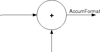
showing that the input data to the sum operations (the addends) retain
their format word length and fraction length from previous operations. The
addition process uses the existing input formats and then casts the output
to the format defined by AccumFormat. Thus the output
data has the word length and fraction length defined by
AccumWordLength and
AccumFracLength.
When CastBeforeSum is true, sum
elements in filter signal flow diagrams look like this:
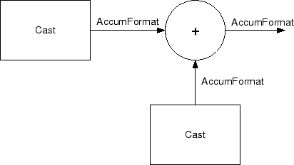
showing that the input data gets recast to the accumulator format word
length and fraction length (AccumFormat) before the sum operation occurs.
The data output by the addition operation has the word length and fraction
length defined by AccumWordLength and
AccumFracLength.
CoeffAutoScale
How the filter represents the filter coefficients depends on the property
value of CoeffAutoScale. When you create a
dfilt object, you use coefficients in double-precision
format. Converting the dfilt object to fixed-point arithmetic
forces the coefficients into a fixed-point representation. The representation
the filter uses depends on whether the value of
CoeffAutoScale is true or
false.
CoeffAutoScale=truemeans the filter chooses the fraction length to maintain the value of the coefficients as close to the double-precision values as possible. When you change the word length applied to the coefficients, the filter object changes the fraction length to try to accommodate the change.trueis the default setting.CoeffAutoScale=falseremoves the automatic scaling of the fraction length for the coefficients and exposes the property that controls the coefficient fraction length so you can change it. For example, if the filter is a direct form FIR filter, settingCoeffAutoScale=falseexposes theNumFracLengthproperty that specifies the fraction length applied to numerator coefficients. If the filter is an IIR filter, settingCoeffAutoScale=falseexposes both theNumFracLengthandDenFracLengthproperties.
Here is an example of using CoeffAutoScale with a direct
form filter.
hd2=dfilt.dffir([0.3 0.6 0.3])

hd2 =

         FilterStructure: 'Direct-Form FIR'
              Arithmetic: 'double'
               Numerator: [0.3000 0.6000 0.3000]
        PersistentMemory: false
                  States: [2x1 double]

hd2.arithmetic='fixed'

hd2 =

         FilterStructure: 'Direct-Form FIR'
              Arithmetic: 'fixed'
               Numerator: [0.3000 0.6000 0.3000]
        PersistentMemory: false
                  States: [1x1 embedded.fi]

         CoeffWordLength: 16
          CoeffAutoScale: true
                  Signed: true

         InputWordLength: 16
         InputFracLength: 15

        OutputWordLength: 16
              OutputMode: 'AvoidOverflow'

             ProductMode: 'FullPrecision'

         AccumWordLength: 40
           CastBeforeSum: true

               RoundMode: 'convergent'
            OverflowMode: 'wrap'
To this point, the filter coefficients retain the original values from when
you created the filter as shown in the Numerator property.
Now change the CoeffAutoScale property value from
true to false.
hd2.coeffautoScale=false

hd2 =

         FilterStructure: 'Direct-Form FIR'
              Arithmetic: 'fixed'
               Numerator: [0.3000 0.6000 0.3000]
        PersistentMemory: false
                  States: [1x1 embedded.fi]

         CoeffWordLength: 16
          CoeffAutoScale: false
           NumFracLength: 15
                  Signed: true

         InputWordLength: 16
         InputFracLength: 15

        OutputWordLength: 16
              OutputMode: 'AvoidOverflow'

             ProductMode: 'FullPrecision'

         AccumWordLength: 40
           CastBeforeSum: true

               RoundMode: 'convergent'
            OverflowMode: 'wrap'
With the NumFracLength property now available, change the
word length to 5 bits.
Notice the coefficient values. Setting CoeffAutoScale to
false removes the automatic fraction length adjustment
and the filter coefficients cannot be represented by the current format of [5
15] — a word length of 5 bits, fraction length of 15 bits.
hd2.coeffwordlength=5

hd2 =

         FilterStructure: 'Direct-Form FIR'
              Arithmetic: 'fixed'
               Numerator: [4.5776e-004 4.5776e-004 4.5776e-004]
        PersistentMemory: false
                  States: [1x1 embedded.fi]

         CoeffWordLength: 5
          CoeffAutoScale: false
           NumFracLength: 15
                  Signed: true

         InputWordLength: 16
         InputFracLength: 15

        OutputWordLength: 16
              OutputMode: 'AvoidOverflow'

             ProductMode: 'FullPrecision'

         AccumWordLength: 40
           CastBeforeSum: true

               RoundMode: 'convergent'
            OverflowMode: 'wrap'
Restoring CoeffAutoScale to true goes
some way to fixing the coefficient values. Automatically scaling the coefficient
fraction length results in setting the fraction length to 4 bits. You can check
this with get(hd2) as shown below.
hd2.coeffautoScale=true

hd2 =

         FilterStructure: 'Direct-Form FIR'
              Arithmetic: 'fixed'
               Numerator: [0.3125 0.6250 0.3125]
        PersistentMemory: false
                  States: [1x1 embedded.fi]

         CoeffWordLength: 5
          CoeffAutoScale: true
                  Signed: true

         InputWordLength: 16
         InputFracLength: 15

        OutputWordLength: 16
              OutputMode: 'AvoidOverflow'

             ProductMode: 'FullPrecision'

         AccumWordLength: 40
           CastBeforeSum: true

               RoundMode: 'convergent'
            OverflowMode: 'wrap'

get(hd2)
        PersistentMemory: false
FilterStructure: 'Direct-Form FIR'
                  States: [1x1 embedded.fi]
               Numerator: [0.3125 0.6250 0.3125]
              Arithmetic: 'fixed'
         CoeffWordLength: 5
          CoeffAutoScale: 1
                  Signed: 1
               RoundMode: 'convergent'
            OverflowMode: 'wrap'
         InputWordLength: 16
         InputFracLength: 15
        OutputWordLength: 16
              OutputMode: 'AvoidOverflow'
             ProductMode: 'FullPrecision'
           NumFracLength: 4
        OutputFracLength: 12
       ProductWordLength: 21
       ProductFracLength: 19
         AccumWordLength: 40
         AccumFracLength: 19
           CastBeforeSum: 1
Clearly five bits is not enough to represent the coefficients accurately.
CoeffFracLength
Fixed-point scalar filters that you create using dfilt.scalar use this property
to define the fraction length applied to the scalar filter coefficients. Like
the coefficient-fraction-length-related properties for the FIR, lattice, and IIR
filters, CoeffFracLength is not displayed for scalar filters
until you set CoeffAutoScale to false.
Once you change the automatic scaling you can set the fraction length for the
coefficients to any value you require.
As with all fraction length properties, the value you enter here can be any
negative or positive integer, or zero. Fraction length can be larger than the
associated word length, as well. By default, the value is 14 bits, with the
CoeffWordlength of 16 bits.
CoeffWordLength
One primary consideration in developing filters for hardware is the length of
a data word. CoeffWordLength defines the word length for
these data storage and arithmetic locations:
Numerator and denominator filter coefficients
Tap sum in
dfilt.dfsymfiranddfilt.dfasymfirfilter objectsSection input, multiplicand, and state values in direct-form SOS filter objects such as
dfilt.df1tanddfilt.df2Scale values in second-order filters
Lattice and ladder coefficients in lattice filter objects, such as
dfilt.latticearmaanddfilt.latticemamaxGain in
dfilt.scalar
Setting this property value controls the word length for the data listed. In most cases, the data words in this list have separate fraction length properties to define the associated fraction lengths.
Any positive, integer word length works here, limited by the machine you use to develop your filter and the hardware you use to deploy your filter.
DenAccumFracLength
Filter structures df1, df1t,
df2, and df2t that use
fixed arithmetic have this property that defines the
fraction length applied to denominator coefficients in the accumulator. In
combination with AccumWordLength, the properties fully
specify how the accumulator outputs data stored there.
As with all fraction length properties,
DenAccumFracLength can be any integer, including
integers larger than AccumWordLength, and positive or
negative integers. To be able to change the property value for this property,
you set FilterInternals to
SpecifyPrecision.
DenFracLength
Property DenFracLength contains the value that specifies
the fraction length for the denominator coefficients for your filter.
DenFracLength specifies the fraction length used to
interpret the data stored in C. Used in combination with
CoeffWordLength, these two properties define the
interpretation of the coefficients stored in the vector that contains the
denominator coefficients.
As with all fraction length properties, the value you enter here can be any
negative or positive integer, or zero. Fraction length can be larger than the
associated word length, as well. By default, the value is 15 bits, with the
CoeffWordLength of 16 bits.
Denominator
The denominator coefficients for your IIR filter, taken from the prototype you start with, are stored in this property. Generally this is a 1-by-N array of data in double format, where N is the length of the filter.
All IIR filter objects include Denominator, except the
lattice-based filters which store their coefficients in the
Lattice property, and second-order section filters,
such as dfilt.df1tsos, which use the
SosMatrix property to hold the coefficients for the
sections.
DenProdFracLength
A property of all of the direct form IIR dfilt objects,
except the ones that implement second-order sections,
DenProdFracLength specifies the fraction length applied
to data output from product operations that the filter performs on denominator
coefficients.
Looking at the signal flow diagram for the dfilt.df1t filter, for example,
you see that denominators and numerators are handled separately. When you set
ProductMode to SpecifyPrecision, you
can change the DenProdFracLength setting manually. Otherwise,
for multiplication operations that use the denominator coefficients, the filter
sets the fraction length as defined by the ProductMode
setting.
DenStateFracLength
When you look at the flow diagram for the dfilt.df1sos filter object, the
states associated with denominator coefficient operations take the fraction
length from this property. In combination with the
DenStateWordLength property, these properties fully
specify how the filter interprets the states.
As with all fraction length properties, the value you enter here can be any
negative or positive integer, or zero. Fraction length can be larger than the
associated word length, as well. By default, the value is 15 bits, with the
DenStateWordLength of 16 bits.
DenStateWordLength
When you look at the flow diagram for the dfilt.df1sos filter object, the
states associated with the denominator coefficient operations take the data
format from this property and the DenStateFracLength
property. In combination, these properties fully specify how the filter
interprets the state it uses.
By default, the value is 16 bits, with the
DenStateFracLength of 15 bits.
FilterInternals
Similar to the FilterInternals pane in FDATool, this property controls whether
the filter sets the output word and fraction lengths automatically, and the
accumulator word and fraction lengths automatically as well, to maintain the
best precision results during filtering. The default value,
FullPrecision, sets automatic word and fraction length
determination by the filter. Setting FilterInternals to
SpecifyPrecision exposes the output and accumulator
related properties so you can set your own word and fraction lengths for them.
Note that
FilterStructure
Every dfilt object has a
FilterStructure property. This is a read-only property
containing a character vector that declares the structure of the filter object
you created.
When you construct filter objects, the FilterStructure
property value is returned containing one of the character vectors shown in the
following table. Property FilterStructure indicates the
filter architecture and comes from the constructor you use to create the
filter.
After you create a filter object, you cannot change the
FilterStructure property value. To make filters that
use different structures, you construct new filters using the appropriate
methods, or use convert to switch to a new
structure.
Default value. Since this depends on the constructor you use and the constructor includes the filter structure definition, there is no default value. When you try to create a filter without specifying a structure, MATLAB returns an error.
Filter Constructor Name | FilterStructure Property and Filter Type |
|---|---|
| Direct form I |
| Direct form I filter implemented using second-order sections |
| Direct form I transposed |
| Direct form II |
| Direct form II filter implemented using second order sections |
| Direct form II transposed |
| Antisymmetric finite impulse response (FIR). Even and odd forms. |
| Direct form FIR |
| Direct form FIR transposed |
| Lattice allpass |
| Lattice autoregressive (AR) |
| Lattice moving average (MA) minimum phase |
| Lattice moving average (MA) maximum phase |
| Lattice ARMA |
| Symmetric FIR. Even and odd forms |
| Scalar |
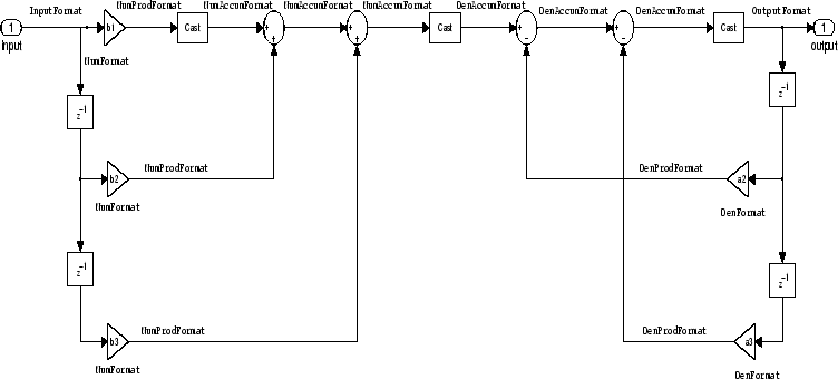
Filter Structures with Quantizations Shown in Place. To help you understand how and where the quantizations occur in filter
structures in this toolbox, the figure below shows the structure for a
Direct Form II filter, including the quantizations (fixed-point formats)
that compose part of the fixed-point filter. You see that one or more
quantization processes, specified by the *format label, accompany each
filter element, such as a delay, product, or summation element. The input to
or output from each element reflects the result of applying the associated
quantization as defined by the word length and fraction length format.
Wherever a particular filter element appears in a filter structure, recall
the quantization process that accompanies the element as it appears in this
figure. Each filter reference page, such as the dfilt.df2 reference page,
includes the signal flow diagram showing the formatting elements that define
the quantizations that occur throughout the filter flow.
For example, a product quantization, either numerator or denominator,
follows every product (gain) element and a sum quantization, also either
numerator or denominator, follows each sum element. The figure shows the
Arithmetic property value set to
fixed.
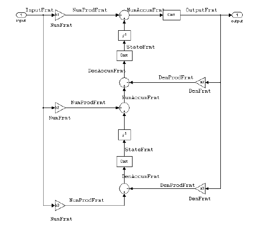
df2 IIR Filter Structure Including the Formatting Objects, with Arithmetic Property Value fixed

When your df2 filter uses the
Arithmetic property set to
fixed, the filter structure contains the formatting
features shown in the diagram. The formats included in the structure are
fixed-point objects that include properties to set various word and fraction
length formats. For example, the NumFormat or
DenFormat properties of the fixed-point arithmetic
filter set the properties for quantizing numerator or denominator
coefficients according to word and fraction length settings.
When the leading denominator coefficient a(1) in your filter is not 1, choose it to be a power of two so that a shift replaces the multiply that would otherwise be used.
Fixed-Point Arithmetic Filter Structures. You choose among several filter structures when you create fixed-point filters. You can also specify filters with single or multiple cascaded sections of the same type. Because quantization is a nonlinear process, different fixed-point filter structures produce different results.
To specify the filter structure, you select the appropriate
dfilt.structure method to
construct your filter. Refer to the function reference information for
dfilt and set for details on setting
property values for quantized filters.
The figures in the following subsections of this section serve as aids to help you determine how to enter your filter coefficients for each filter structure. Each subsection contains an example for constructing a filter of the given structure.
Scale factors for the input and output for the filters do not appear in
the block diagrams. The default filter structures do not include, nor
assume, the scale factors. For filter scaling information, refer to
scale in the Help
system.
About the Filter Structure Diagrams. In the diagrams that accompany the following filter structure descriptions, you see the active operators that define the filter, such as sums and gains, and the formatting features that control the processing in the filter. Notice also that the coefficients are labeled in the figure. This tells you the order in which the filter processes the coefficients.
While the meaning of the block elements is straightforward, the labels for
the formats that form part of the filter are less clear. Each figure
includes text in the form labelFormat that
represents the existence of a formatting feature at that point in the
structure. The Format stands for formatting
object and the label specifies the data that the
formatting object affects.
For example, in the dfilt.df2 filter shown
above, the entries
InputFormat and OutputFormat are
the formats applied, that is the word length and fraction length, to the
filter input and output data. For example, filter properties like
OutputWordLength and
InputWordLength specify values that control filter
operations at the input and output points in the structure and are
represented by the formatting objects InputFormat and
OutputFormat shown in the filter structure
diagrams.
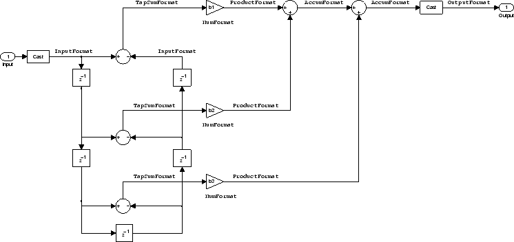
Direct Form I Filter Structure. The following figure depicts the direct form I filter
structure that directly realizes a transfer function with a second-order
numerator and denominator. The numerator coefficients are numbered
b(i), i =1, 2,
3; the denominator coefficients are numbered
a(i), i = 1, 2,
3; and the states (used for initial and final state values in filtering) are
labeled z(i). In the figure, the
Arithmetic property is set to
fixed.
Example — Specifying a Direct Form I Filter. You can specify a second-order direct form I structure for a quantized
filter hq with the following code.
b = [0.3 0.6 0.3];
a = [1 0 0.2];
hq = dfilt.df1(b,a);
To create the fixed-point filter, set the Arithmetic
property to fixed as shown here.
set(hq,'arithmetic','fixed');
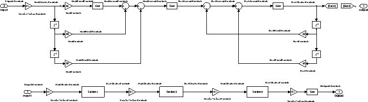
Direct Form I Filter Structure With Second-Order Sections. The following figure depicts a direct form I filter
structure that directly realizes a transfer function with a second-order
numerator and denominator and second-order sections. The numerator
coefficients are numbered b(i),
i =1, 2, 3; the denominator coefficients are numbered
a(i), i = 1, 2,
3; and the states (used for initial and final state values in filtering) are
labeled z(i). In the figure, the
Arithmetic property is set to
fixed to place the filter in fixed-point mode.
Example — Specifying a Direct Form I Filter with Second-Order
Sections. You can specify an eighth-order direct form I structure for a quantized
filter hq with the following code.
b = [0.3 0.6 0.3];
a = [1 0 0.2];
hq = dfilt.df1sos(b,a);
To create the fixed-point filter, set the Arithmetic
property to fixed, as shown here.
set(hq,'arithmetic','fixed');
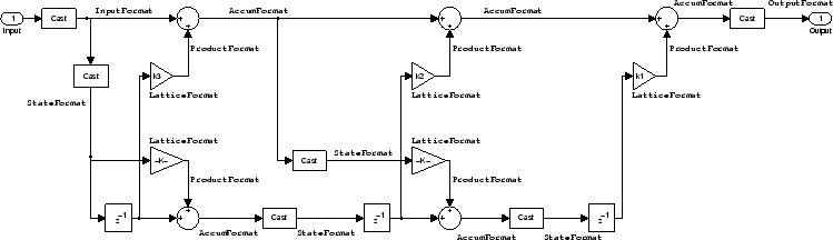
Direct Form I Transposed Filter Structure. The next signal flow diagram depicts a direct form I
transposed filter structure that directly realizes a
transfer function with a second-order numerator and denominator. The
numerator coefficients are b(i),
i = 1, 2, 3; the denominator coefficients are
a(i), i = 1, 2,
3; and the states (used for initial and final state values in filtering) are
labeled z(i). With the
Arithmetic property value set to
fixed, the figure shows the filter with the
properties indicated.

Example — Specifying a Direct Form I Transposed Filter. You can specify a second-order direct form I transposed filter
structure for a quantized filter hq with the following
code.
b = [0.3 0.6 0.3];
a = [1 0 0.2];
hq = dfilt.df1t(b,a);
set(hq,'arithmetic','fixed');
Direct Form II Filter Structure. The following graphic depicts a direct form II filter
structure that directly realizes a transfer function with a second-order
numerator and denominator. In the figure, the
Arithmetic property value is
fixed. Numerator coefficients are named
b(i); denominator coefficients are
named a(i), i = 1,
2, 3; and the states (used for initial and final state values in filtering)
are named z(i).
Use the method dfilt.df2 to construct a quantized
filter whose FilterStructure property is
Direct-Form II.
Example — Specifying a Direct Form II Filter. You can specify a second-order direct form II filter structure for a
quantized filter hq with the following code.
b = [0.3 0.6 0.3];
a = [1 0 0.2];
hq = dfilt.df2(b,a);
hq.arithmetic = 'fixed'
To convert your initial double-precision filter hq to a
quantized or fixed-point filter, set the Arithmetic
property to fixed, as shown.
Direct Form II Filter Structure With Second-Order Sections
The following figure depicts direct form II filter
structure using second-order sections that directly realizes a transfer
function with a second-order numerator and denominator sections. In the
figure, the Arithmetic property value is
fixed. Numerator coefficients are labeled
b(i); denominator coefficients are
labeled a(i), i =
1, 2, 3; and the states (used for initial and final state values in
filtering) are labeled z(i).
Use the method dfilt.df2sos to construct a quantized
filter whose FilterStructure property is
Direct-Form II.
Example — Specifying a Direct Form II Filter with Second-Order
Sections. You can specify a tenth-order direct form II filter structure that uses
second-order sections for a quantized filter hq with the
following code.
b = [0.3 0.6 0.3];
a = [1 0 0.2];
hq = dfilt.df2sos(b,a);
hq.arithmetic = 'fixed'
To convert your prototype double-precision filter hq to
a fixed-point filter, set the Arithmetic property to
fixed, as shown.
Direct Form II Transposed Filter Structure. The following figure depicts the direct form II
transposed filter structure that directly realizes
transfer functions with a second-order numerator and denominator. The
numerator coefficients are labeled
b(i), the denominator coefficients are
labeled a(i), i =
1, 2, 3, and the states (used for initial and final state values in
filtering) are labeled z(i). In the
first figure, the Arithmetic property value is
fixed.
Use the constructor dfilt.df2t to specify the
value of the FilterStructure property for a filter with
this structure that you can convert to fixed-point filtering.
Example — Specifying a Direct Form II Transposed Filter. Specifying or constructing a second-order direct form II transposed filter
for a fixed-point filter hq starts with the following
code to define the coefficients and construct the filter.
b = [0.3 0.6 0.3];
a = [1 0 0.2];
hd = dfilt.df2t(b,a);
Now create the fixed-point filtering version of the filter from
hd, which is floating point.
hq = set(hd,'arithmetic','fixed');
Direct Form Antisymmetric FIR Filter Structure (Any Order). The following figure depicts a direct form antisymmetric FIR
filter structure that directly realizes a second-order
antisymmetric FIR filter. The filter coefficients are labeled
b(i), and the initial and final state values in
filtering are labeled z(i). This
structure reflects the Arithmetic property set to
fixed.
Use the method dfilt.dfasymfir to construct the filter,
and then set the Arithmetic property to
fixed to convert to a fixed-point filter with this
structure.
Example — Specifying an Odd-Order Direct Form Antisymmetric FIR
Filter. Specify a fifth-order direct form antisymmetric FIR filter structure for a
fixed-point filter hq with the following code.
b = [-0.008 0.06 -0.44 0.44 -0.06 0.008];
hq = dfilt.dfasymfir(b);
set(hq,'arithmetic','fixed')

hq

hq =

         FilterStructure: 'Direct-Form Antisymmetric FIR'
              Arithmetic: 'fixed'
               Numerator: [-0.0080 0.0600 -0.4400 0.4400 -0.0600 0.0080]
        PersistentMemory: false
                  States: [1x1 fi object]

         CoeffWordLength: 16
          CoeffAutoScale: true
                  Signed: true

         InputWordLength: 16
         InputFracLength: 15

        OutputWordLength: 16
              OutputMode: 'AvoidOverflow'

              TapSumMode: 'KeepMSB'
        TapSumWordLength: 17

             ProductMode: 'FullPrecision'

         AccumWordLength: 40

           CastBeforeSum: true
               RoundMode: 'convergent'
            OverflowMode: 'wrap'

         InheritSettings: false
Example — Specifying an Even-Order Direct Form Antisymmetric FIR
Filter. You can specify a fourth-order direct form antisymmetric FIR filter
structure for a fixed-point filter hq with the following
code.
b = [-0.01 0.1 0.0 -0.1 0.01];
hq = dfilt.dfasymfir(b);
hq.arithmetic='fixed'
hq =
FilterStructure: 'Direct-Form Antisymmetric FIR'
Arithmetic: 'fixed'
Numerator: [-0.0100 0.1000 0 -0.1000 0.0100]
PersistentMemory: false
States: [1x1 fi object]
CoeffWordLength: 16
CoeffAutoScale: true
Signed: true
InputWordLength: 16
InputFracLength: 15
OutputWordLength: 16
OutputMode: 'AvoidOverflow'
TapSumMode: 'KeepMSB'
TapSumWordLength: 17
ProductMode: 'FullPrecision'
AccumWordLength: 40
CastBeforeSum: true
RoundMode: 'convergent'
OverflowMode: 'wrap'
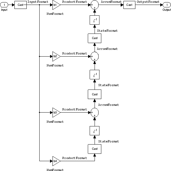
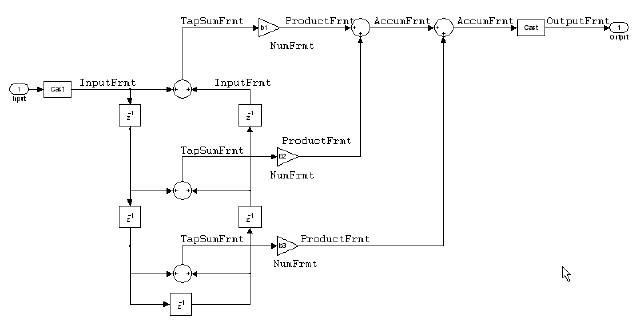
InheritSettings: false Direct Form Finite Impulse Response (FIR) Filter Structure. In the next figure, you see the signal flow graph for a direct
form finite impulse response (FIR) filter structure that
directly realizes a second-order FIR filter. The filter coefficients are
b(i), i = 1, 2,
3, and the states (used for initial and final state values in filtering) are
z(i). To generate the figure, set
the Arithmetic property to fixed
after you create your prototype filter in double-precision
arithmetic.

Use the dfilt.dffir method to generate a filter that
uses this structure.
Example — Specifying a Direct Form FIR Filter. You can specify a second-order direct form FIR filter structure for a
fixed-point filter hq with the following code.
b = [0.05 0.9 0.05];
hd = dfilt.dffir(b);
hq = set(hd,'arithmetic','fixed');
Direct Form FIR Transposed Filter Structure. This figure uses the filter coefficients labeled b(i), i = 1, 2, 3, and states (used for initial and final state values in filtering) are labeled z(i). These depict a direct form finite impulse response (FIR) transposed filter structure that directly realizes a second-order FIR filter.
With the Arithmetic property set to
fixed, your filter matches the figure. Using the
method dfilt.dffirt returns a double-precision filter
that you convert to a fixed-point filter.
Example — Specifying a Direct Form FIR Transposed Filter. You can specify a second-order direct form FIR transposed filter structure
for a fixed-point filter hq with the following
code.
b = [0.05 0.9 0.05];
hd=dfilt.dffirt(b);
hq = copy(hd);
hq.arithmetic = 'fixed';
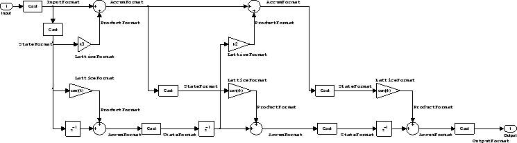
Lattice Allpass Filter Structure. The following figure depicts the lattice allpass filter structure. The pictured structure directly realizes third-order lattice allpass filters using fixed-point arithmetic. The filter reflection coefficients are labeled k1(i), i = 1, 2, 3. The states (used for initial and final state values in filtering) are labeled z(i).

To create a quantized filter that uses the lattice allpass structure shown
in the figure, use the dfilt.latticeallpass method and
set the Arithmetic property to
fixed.
Example — Specifying a Lattice Allpass Filter. You can create a third-order lattice allpass filter structure for a
quantized filter hq with the following code.
k = [.66 .7 .44];
hd=dfilt.latticeallpass(k);
set(hq,'arithmetic','fixed');
Lattice Moving Average Maximum Phase Filter Structure. In the next figure you see a lattice moving average maximum phase filter structure. This signal flow diagram directly realizes a third-order lattice moving average (MA) filter with the following phase form depending on the initial transfer function:
When you start with a minimum phase transfer function, the upper branch of the resulting lattice structure returns a minimum phase filter. The lower branch returns a maximum phase filter.
When your transfer function is neither minimum phase nor maximum phase, the lattice moving average maximum phase structure will not be maximum phase.
When you start with a maximum phase filter, the resulting lattice filter is maximum phase also.
The filter reflection coefficients are labeled
k(i), i = 1, 2,
3. The states (used for initial and final state values in filtering) are
labeled z(i). In the figure, we set
the Arithmetic property to fixed to
reveal the fixed-point arithmetic format features that control such options
as word length and fraction length.
Example — Constructing a Lattice Moving Average Maximum Phase
Filter. Constructing a fourth-order lattice MA maximum phase filter structure for
a quantized filter hq begins with the following
code.
k = [.66 .7 .44 .33];
hd=dfilt.latticemamax(k);
Lattice Autoregressive (AR) Filter Structure. The method dfilt.latticear directly realizes lattice
autoregressive filters in the toolbox. The following figure depicts the
third-order lattice autoregressive (AR) filter
structure — with the Arithmetic property equal
to fixed. The filter reflection coefficients are labeled
k(i), i = 1, 2,
3, and the states (used for initial and final state values in filtering) are
labeled z(i).

Example — Specifying a Lattice AR Filter. You can specify a third-order lattice AR filter structure for a quantized
filter hq with the following code.
k = [.66 .7 .44];
hd=dfilt.latticear(k);
hq.arithmetic = 'custom';
Lattice Moving Average (MA) Filter Structure for Minimum Phase. The following figures depict lattice moving average
(MA) filter structures that directly realize third-order
lattice MA filters for minimum phase. The filter reflection coefficients are
labeled k(i), (i).
= 1, 2, 3, and the states (used for initial and final state values in
filtering) are labeled z(i). Setting
the Arithmetic property of the filter to
fixed results in a fixed-point filter that matches
the figure.
This signal flow diagram directly realizes a third-order lattice moving average (MA) filter with the following phase form depending on the initial transfer function:
When you start with a minimum phase transfer function, the upper branch of the resulting lattice structure returns a minimum phase filter. The lower branch returns a minimum phase filter.
When your transfer function is neither minimum phase nor maximum phase, the lattice moving average minimum phase structure will not be minimum phase.
When you start with a minimum phase filter, the resulting lattice filter is minimum phase also.
The filter reflection coefficients are labeled
k((i).), i = 1,
2, 3. The states (used for initial and final state values in filtering) are
labeled z((i).). This figure shows the
filter structure when the Arithmetic property is set to
fixed to reveal the fixed-point arithmetic format
features that control such options as word length and fraction
length.
Example — Specifying a Minimum Phase Lattice MA Filter. You can specify a third-order lattice MA filter structure for minimum phase applications using variations of the following code.
k = [.66 .7 .44];
hd=dfilt.latticemamin(k);
set(hq,'arithmetic','fixed');
Lattice Autoregressive Moving Average (ARMA) Filter Structure. The figure below depicts a lattice autoregressive moving average (ARMA) filter structure that directly realizes a fourth-order lattice ARMA filter. The filter reflection coefficients are labeled k(i), (i). = 1, ..., 4; the ladder coefficients are labeled v(i), (i). = 1, 2, 3; and the states (used for initial and final state values in filtering) are labeled z(i).

Example — Specifying an Lattice ARMA Filter. The following code specifies a fourth-order lattice ARMA filter structure
for a quantized filter hq, starting from
hd, a floating-point version of the filter.
k = [.66 .7 .44 .66];
v = [1 0 0];
hd=dfilt.latticearma(k,v);
hq.arithmetic = 'fixed';
Direct Form Symmetric FIR Filter Structure (Any Order). Shown in the next figure, you see signal flow that depicts a
direct form
symmetric FIR filter structure that directly realizes a
fifth-order direct form symmetric FIR filter. Filter coefficients are
labeled b(i), i =
1, ..., n, and states (used for initial and final state
values in filtering) are labeled z(i).
Showing the filter structure used when you select fixed
for the Arithmetic property value, the first figure
details the properties in the filter object.
Example — Specifying an Odd-Order Direct Form Symmetric FIR
Filter. By using the following code in MATLAB, you can specify a fifth-order direct form symmetric FIR
filter for a fixed-point filter hq:
b = [-0.008 0.06 0.44 0.44 0.06 -0.008];
hd=dfilt.dfsymfir(b);
set(hq,'arithmetic','fixed');
Assigning Filter Coefficients. The syntax you use to assign filter coefficients for your floating-point or fixed-point filter depends on the structure you select for your filter.
Converting Filters Between Representations. Filter conversion functions in this toolbox and in Signal Processing Toolbox software let you convert filter transfer functions to other filter forms, and from other filter forms to transfer function form. Relevant conversion functions include the following functions.
Conversion Function | Description |
|---|---|
Converts from a coupled allpass filter to a transfer function. | |
Converts from a lattice coupled allpass filter to a transfer function. | |
Convert a discrete-time filter from one filter structure to another. | |
Converts quantized filters to create second-order sections. We recommend this method for converting quantized filters to second-order sections. | |
Converts from a transfer function to a coupled allpass filter. | |
Converts from a transfer function to a lattice coupled allpass filter. | |
Converts from a transfer function to a lattice filter. | |
Converts from a transfer function to a second-order section form. | |
Converts from a transfer function to state-space form. | |
Converts from a rational transfer function to its factored (single section) form (zero-pole-gain form). | |
Converts a zero-pole-gain form to a second-order section form. | |
Conversion of zero-pole-gain form to a state-space form. | |
Conversion of zero-pole-gain form to transfer functions of multiple order sections. |
Note that these conversion routines do not apply to
dfilt objects.
The function convert is a special case
— when you use convert to change the filter structure of a
fixed-point filter, you lose all of the filter states and settings. Your new
filter has default values for all properties, and it is not
fixed-point.
To demonstrate the changes that occur, convert a fixed-point direct form I transposed filter to direct form II structure.
hd=dfilt.df1t

hd =

         FilterStructure: 'Direct-Form I Transposed'
              Arithmetic: 'double'
               Numerator: 1
             Denominator: 1
        PersistentMemory: false
                  States: Numerator:  [0x0 double]
                          Denominator:[0x0 double]


hd.arithmetic='fixed'
hd =

         FilterStructure: 'Direct-Form I Transposed'
              Arithmetic: 'fixed'
               Numerator: 1
             Denominator: 1
        PersistentMemory: false
                  States: Numerator:  [0x0 fi]
                          Denominator:[0x0 fi]

convert(hd,'df2')

Warning: Using reference filter for structure conversion.
Fixed-point attributes will not be converted.

ans =

         FilterStructure: 'Direct-Form II'
              Arithmetic: 'double'
               Numerator: 1
             Denominator: 1
        PersistentMemory: false
                  States: [0x1 double]
You can specify a filter with L sections of arbitrary order by
Gain
dfilt.scalar filters have a gain value stored in the
gain property. By default the gain value is one
— the filter acts as a wire.
InputFracLength
InputFracLength defines the fraction length assigned to the
input data for your filter. Used in tandem with
InputWordLength, the pair defines the data format for
input data you provide for filtering.
As with all fraction length properties in dfilt objects,
the value you enter here can be any negative or positive integer, or zero.
Fraction length can be larger than the associated word length, in this case
InputWordLength, as well.
InputWordLength
Specifies the number of bits your filter uses to represent your input data.
Your word length option is limited by the arithmetic you choose — up to
32 bits for double, float, and
fixed. Setting Arithmetic to
single (single-precision floating-point) limits word
length to 16 bits. The default value is 16 bits.
Ladder
Included as a property in dfilt.latticearma filter objects,
Ladder contains the denominator coefficients that form an
IIR lattice filter object. For instance, the following code creates a high pass
filter object that uses the lattice ARMA structure.
[b,a]=cheby1(5,.5,.5,'high')

b =

    0.0282   -0.1409    0.2817   -0.2817    0.1409   -0.0282


a =

    1.0000    0.9437    1.4400    0.9629    0.5301    0.1620

hd=dfilt.latticearma(b,a)

hd =

         FilterStructure: [1x44 char]
              Arithmetic: 'double'
                 Lattice: [1x6 double]
                  Ladder: [1 0.9437 1.4400 0.9629 0.5301 0.1620]
     PersistentMemory: false
                  States: [6x1 double]

hd.arithmetic='fixed'

hd =

         FilterStructure: [1x44 char]
              Arithmetic: 'fixed'
                 Lattice: [1x6 double]
                  Ladder: [1 0.9437 1.4400 0.9629 0.5301 0.1620]
     PersistentMemory: false
                  States: [1x1 embedded.fi]

         CoeffWordLength: 16
          CoeffAutoScale: true
                  Signed: true

         InputWordLength: 16
         InputFracLength: 15

        OutputWordLength: 16
              OutputMode: 'AvoidOverflow'

         StateWordLength: 16
         StateFracLength: 15

             ProductMode: 'FullPrecision'

         AccumWordLength: 40
           CastBeforeSum: true

               RoundMode: 'convergent'
            OverflowMode: 'wrap'
LadderAccumFracLength
Autoregressive, moving average lattice filter objects
(lattticearma) use ladder coefficients to define the
filter. In combination with LadderFracLength and
CoeffWordLength, these three properties specify or
reflect how the accumulator outputs data stored there. As with all fraction
length properties, LadderAccumFracLength can be any integer,
including integers larger than AccumWordLength, and positive
or negative integers. The default value is 29 bits.
LadderFracLength
To let you control the way your latticearma filter
interprets the denominator coefficients, LadderFracLength
sets the fraction length applied to the ladder coefficients for your filter. The
default value is 14 bits.
As with all fraction length properties, LadderFracLength
can be any integer, including integers larger than
AccumWordLength, and positive or negative integers.
Lattice
When you create a lattice-based IIR filter, your numerator coefficients (from
your IIR prototype filter or the default dfilt lattice
filter function) get stored in the Lattice property of the
dfilt object. The properties
CoeffWordLength and
LatticeFracLength define the data format the object
uses to represent the lattice coefficients. By default, lattice coefficients are
in double-precision format.
LatticeAccumFracLength
Lattice filter objects (latticeallpass,
latticearma, latticemamax, and
latticemamin) use lattice coefficients to define the
filter. In combination with LatticeFracLength and
CoeffWordLength, these three properties specify how the
accumulator outputs lattice coefficient-related data stored there. As with all
fraction length properties, LatticeAccumFracLength can be
any integer, including integers larger than AccumWordLength,
and positive or negative integers. By default, the property is set to 31
bits.
LatticeFracLength
To let you control the way your filter interprets the denominator
coefficients, LatticeFracLength sets the fraction length
applied to the lattice coefficients for your lattice filter. When you create the
default lattice filter, LatticeFracLength is 16
bits.
As with all fraction length properties, LatticeFracLength
can be any integer, including integers larger than
CoeffWordLength, and positive or negative integers.
MultiplicandFracLength
Each input data element for a multiply operation has both word length and
fraction length to define its representation.
MultiplicandFracLength sets the fraction length to use
when the filter object performs any multiply operation during filtering. For
default filters, this is set to 15 bits.
As with all word and fraction length properties,
MultiplicandFracLength can be any integer, including
integers larger than CoeffWordLength, and positive or
negative integers.
MultiplicandWordLength
Each input data element for a multiply operation has both word length and
fraction length to define its representation.
MultiplicandWordLength sets the word length to use when
the filter performs any multiply operation during filtering. For default
filters, this is set to 16 bits. Only the df1t and
df1tsos filter objects include the
MultiplicandFracLength property.
Only the df1t and df1tsos filter objects
include the MultiplicandWordLength property.
NumAccumFracLength
Filter structures df1, df1t,
df2, and df2t that use
fixed arithmetic have this property that defines the
fraction length applied to numerator coefficients in output from the
accumulator. In combination with AccumWordLength, the
NumAccumFracLength property fully specifies how the
accumulator outputs numerator-related data stored there.
As with all fraction length properties,
NumAccumFracLength can be any integer, including
integers larger than AccumWordLength, and positive or
negative integers. 30 bits is the default value when you create the filter
object. To be able to change the value for this property, set
FilterInternals for the filter to
SpecifyPrecision.
Numerator
The numerator coefficients for your filter, taken from the prototype you start with or from the default filter, are stored in this property. Generally this is a 1-by-N array of data in double format, where N is the length of the filter.
All of the filter objects include Numerator, except the
lattice-based and second-order section filters, such as
dfilt.latticema and
dfilt.df1tsos.
NumFracLength
Property NumFracLength contains the value that specifies
the fraction length for the numerator coefficients for your filter.
NumFracLength specifies the fraction length used to
interpret the numerator coefficients. Used in combination with
CoeffWordLength, these two properties define the
interpretation of the coefficients stored in the vector that contains the
numerator coefficients.
As with all fraction length properties, the value you enter here can be any
negative or positive integer, or zero. Fraction length can be larger than the
associated word length, as well. By default, the value is 15 bits, with the
CoeffWordLength of 16 bits.
NumProdFracLength
A property of all of the direct form IIR dfilt objects,
except the ones that implement second-order sections,
NumProdFracLength specifies the fraction length applied
to data output from product operations the filter performs on numerator
coefficients.
Looking at the signal flow diagram for the dfilt.df1t filter, for example,
you see that denominators and numerators are handled separately. When you set
ProductMode to SpecifyPrecision, you
can change the NumProdFracLength setting manually.
Otherwise, for multiplication operations that use the numerator coefficients,
the filter sets the word length as defined by the ProductMode
setting.
NumStateFracLength
All the variants of the direct form I structure include the property
NumStateFracLength to store the fraction length applied
to the numerator states for your filter object. By default, this property has
the value 15 bits, with the CoeffWordLength of 16 bits, which
you can change after you create the filter object.
As with all fraction length properties, the value you enter here can be any negative or positive integer, or zero. Fraction length can be larger than the associated word length, as well.
NumStateWordLength
When you look at the flow diagram for the df1sos filter
object, the states associated with the numerator coefficient operations take the
data format from this property and the NumStateFracLength
property. In combination, these properties fully specify how the filter
interprets the state it uses.
As with all fraction length properties, the value you enter here can be any
negative or positive integer, or zero. Fraction length can be larger than the
associated word length, as well. By default, the value is 16 bits, with the
NumStateFracLength of 11 bits.
OutputFracLength
To define the output from your filter object, you need both the word and
fraction lengths. OutputFracLength determines the fraction
length applied to interpret the output data. Combining this with
OutputWordLength fully specifies the format of the
output.
Your fraction length can be any negative or positive integer, or zero. In addition, the fraction length you specify can be larger than the associated word length. Generally, the default value is 11 bits.
OutputMode
Sets the mode the filter uses to scale the filtered (output) data. You have the following choices:
AvoidOverflow— directs the filter to set the property that controls the output data fraction length to avoid causing the data to overflow. In adf2filter, this would be theOutputFracLengthproperty.BestPrecision— directs the filter to set the property that controls the output data fraction length to maximize the precision in the output data. Fordf1tfilters, this is theOutputFracLengthproperty. When you change the word length (OutputWordLength), the filter adjusts the fraction length to maintain the best precision for the new word size.SpecifyPrecision— lets you set the fraction length used by the filtered data. When you select this choice, you can set the output fraction length using theOutputFracLengthproperty to define the output precision.
All filters include this property except the direct form I filter which takes the output format from the filter states.
Here is an example that changes the mode setting to
bestprecision, and then adjusts the word length for the
output.
hd=dfilt.df2

hd =

         FilterStructure: 'Direct-Form II'
              Arithmetic: 'double'
               Numerator: 1
             Denominator: 1
        PersistentMemory: false
                  States: [0x1 double]

hd.arithmetic='fixed'

hd =

         FilterStructure: 'Direct-Form II'
              Arithmetic: 'fixed'
               Numerator: 1
             Denominator: 1
        PersistentMemory: false
                  States: [1x1 embedded.fi]

         CoeffWordLength: 16
          CoeffAutoScale: true
                  Signed: true

         InputWordLength: 16
         InputFracLength: 15

        OutputWordLength: 16
              OutputMode: 'AvoidOverflow'

         StateWordLength: 16
         StateFracLength: 15

             ProductMode: 'FullPrecision'

         AccumWordLength: 40
           CastBeforeSum: true

               RoundMode: 'convergent'
            OverflowMode: 'wrap'

get(hd)
        PersistentMemory: false
FilterStructure: 'Direct-Form II'
                  States: [1x1 embedded.fi]
               Numerator: 1
             Denominator: 1
              Arithmetic: 'fixed'
         CoeffWordLength: 16
          CoeffAutoScale: 1
                  Signed: 1
               RoundMode: 'convergent'
            OverflowMode: 'wrap'
         InputWordLength: 16
         InputFracLength: 15
        OutputWordLength: 16
              OutputMode: 'AvoidOverflow'
             ProductMode: 'FullPrecision'
         StateWordLength: 16
         StateFracLength: 15
           NumFracLength: 14
           DenFracLength: 14
        OutputFracLength: 13
       ProductWordLength: 32
       NumProdFracLength: 29
       DenProdFracLength: 29
         AccumWordLength: 40
      NumAccumFracLength: 29
      DenAccumFracLength: 29
           CastBeforeSum: 1

hd.outputMode='bestprecision'

hd =

         FilterStructure: 'Direct-Form II'
              Arithmetic: 'fixed'
               Numerator: 1
             Denominator: 1
        PersistentMemory: false
                  States: [1x1 embedded.fi]

         CoeffWordLength: 16
          CoeffAutoScale: true
                  Signed: true

         InputWordLength: 16
         InputFracLength: 15

        OutputWordLength: 16
              OutputMode: 'BestPrecision'

         StateWordLength: 16
         StateFracLength: 15

             ProductMode: 'FullPrecision'

         AccumWordLength: 40
           CastBeforeSum: true

               RoundMode: 'convergent'
            OverflowMode: 'wrap'

hd.outputWordLength=8;

get(hd)
        PersistentMemory: false
         FilterStructure: 'Direct-Form II'
                  States: [1x1 embedded.fi]
               Numerator: 1
             Denominator: 1
              Arithmetic: 'fixed'
         CoeffWordLength: 16
          CoeffAutoScale: 1
                  Signed: 1
               RoundMode: 'convergent'
            OverflowMode: 'wrap'
         InputWordLength: 16
         InputFracLength: 15
        OutputWordLength: 8
              OutputMode: 'BestPrecision'
             ProductMode: 'FullPrecision'
         StateWordLength: 16
         StateFracLength: 15
           NumFracLength: 14
           DenFracLength: 14
        OutputFracLength: 5
       ProductWordLength: 32
       NumProdFracLength: 29
       DenProdFracLength: 29
         AccumWordLength: 40
      NumAccumFracLength: 29
      DenAccumFracLength: 29
           CastBeforeSum: 1
Changing the OutputWordLength to 8 bits
caused the filter to change the OutputFracLength to
5 bits to keep the best precision for the output
data.
OutputWordLength
Use the property OutputWordLength to set the word length
used by the output from your filter. Set this property to a value that matches
your intended hardware. For example, some digital signal processors use 32-bit
output so you would set OutputWordLength to
32.
[b,a] = butter(6,.5);
hd=dfilt.df1t(b,a);

set(hd,'arithmetic','fixed')

hd

hd =

         FilterStructure: 'Direct-Form I Transposed'
              Arithmetic: 'fixed'
               Numerator: [1x7 double]
             Denominator: [1 0 0.7777 0 0.1142 0 0.0018]
     PersistentMemory: false
                  States: Numerator:  [6x1 fi]
                          Denominator:[6x1 fi]


         CoeffWordLength: 16
          CoeffAutoScale: true
                  Signed: true

         InputWordLength: 16
         InputFracLength: 15

        OutputWordLength: 16
              OutputMode: 'AvoidOverflow'

  MultiplicandWordLength: 16
  MultiplicandFracLength: 15

         StateWordLength: 16
          StateAutoScale: true

             ProductMode: 'FullPrecision'

         AccumWordLength: 40
           CastBeforeSum: true

               RoundMode: 'convergent'
            OverflowMode: 'wrap'

hd.outputwordLength=32

hd =

         FilterStructure: 'Direct-Form I Transposed'
              Arithmetic: 'fixed'
               Numerator: [1x7 double]
             Denominator: [1 0 0.7777 0 0.1142 0 0.0018]
        PersistentMemory: false
                  States: Numerator:  [6x1 fi]
                          Denominator:[6x1 fi]


         CoeffWordLength: 16
          CoeffAutoScale: true
                  Signed: true

         InputWordLength: 16
         InputFracLength: 15

        OutputWordLength: 32
              OutputMode: 'AvoidOverflow'

  MultiplicandWordLength: 16
  MultiplicandFracLength: 15

         StateWordLength: 16
          StateAutoScale: true

             ProductMode: 'FullPrecision'

         AccumWordLength: 40
           CastBeforeSum: true

               RoundMode: 'convergent'
            OverflowMode: 'wrap'
When you create a filter object, this property starts with the value 16.
OverflowMode
The OverflowMode property is specified as one of the
following two character vectors indicating how to respond to overflows in
fixed-point arithmetic:
'saturate'— saturate overflows.When the values of data to be quantized lie outside of the range of the largest and smallest representable numbers (as specified by the applicable word length and fraction length properties), these values are quantized to the value of either the largest or smallest representable value, depending on which is closest.
saturateis the default value forOverflowMode.'wrap'— wrap all overflows to the range of representable values.When the values of data to be quantized lie outside of the range of the largest and smallest representable numbers (as specified by the data format properties), these values are wrapped back into that range using modular arithmetic relative to the smallest representable number. You can learn more about modular arithmetic in Fixed-Point Designer documentation.
These rules apply to the OverflowMode property.
Applies to the accumulator and output data only.
Does not apply to coefficients or input data. These always saturate the results.
Does not apply to products. Products maintain full precision at all times. Your filters do not lose precision in the products.
Note
Numbers in floating-point filters that extend beyond the dynamic range
overflow to ±inf.
ProductFracLength
After you set ProductMode for a fixed-point filter to
SpecifyPrecision, this property becomes available for you
to change. ProductFracLength sets the fraction length the
filter uses for the results of multiplication operations. Only the FIR filters
such as asymmetric FIRs or lattice autoregressive filters include this dynamic
property.
Your fraction length can be any negative or positive integer, or zero. In addition, the fraction length you specify can be larger than the associated word length. Generally, the default value is 11 bits.
ProductMode
This property, available when your filter is in fixed-point arithmetic mode,
specifies how the filter outputs the results of multiplication operations. All
dfilt objects include this property when they use
fixed-point arithmetic.
When available, you select from one of the following values for
ProductMode:
FullPrecision— means the filter automatically chooses the word length and fraction length it uses to represent the results of multiplication operations. The setting allow the product to retain the precision provided by the inputs (multiplicands) to the operation.KeepMSB— means you specify the word length for representing product operation results. The filter sets the fraction length to discard the LSBs, keep the higher order bits in the data, and maintain the precision.KeepLSB— means you specify the word length for representing the product operation results. The filter sets the fraction length to discard the MSBs, keep the lower order bits, and maintain the precision. Compare to theKeepMSBoption.SpecifyPrecision— means you specify the word length and the fraction length to apply to data output from product operations.
When you switch to fixed-point filtering from floating-point, you are most
likely going to throw away some data bits after product operations in your
filter, perhaps because you have limited resources. When you have to discard
some bits, you might choose to discard the least significant bits (LSB) from a
result since the resulting quantization error would be small as the LSBs carry
less weight. Or you might choose to keep the LSBs because the results have MSBs
that are mostly zero, such as when your values are small relative to the range
of the format in which they are represented. So the options for
ProductMode let you choose how to maintain the
information you need from the accumulator.
For more information about data formats, word length, and fraction length in fixed-point arithmetic, refer to Notes About Fraction Length, Word Length, and Precision.
ProductWordLength
You use ProductWordLength to define the data word length
used by the output from multiplication operations. Set this property to a value
that matches your intended application. For example, the default value is 32
bits, but you can set any word length.
set(hq,'arithmetic','fixed');
set(hq,'ProductWordLength',64);
Note that ProductWordLength applies only to filters whose
Arithmetic property value is
fixed.
PersistentMemory
Determine whether the filter states get restored to their starting values for
each filtering operation. The starting values are the values in place when you
create the filter object. PersistentMemory returns to zero
any state that the filter changes during processing. States that the filter does
not change are not affected. Defaults to false — the
filter does not retain memory about filtering operations from one to the next.
Maintaining memory (setting PersistentMemory to
true) lets you filter large data sets as collections of
smaller subsets and get the same result.
In this example, filter hd first filters data
xtot in one pass. Then you can use hd
to filter x as two separate data sets. The results
ytot and ysec are the same in both
cases.
xtot=[x,x];
ytot=filter(hd,xtot)
ytot =

         0   -0.0003    0.0005   -0.0014    0.0028   -0.0054    0.0092
reset(hm1);  % Clear history of the filter
hm1.PersistentMemory='true';
ysec=[filter(hd,x) filter(hd,x)]

ysec =

         0   -0.0003    0.0005   -0.0014    0.0028   -0.0054    0.0092
This test verifies that ysec (the signal filtered by
sections) is equal to ytot (the entire signal filtered at
once).
RoundMode
The RoundMode property value specifies the rounding
method used for quantizing numerical values. Specify the
RoundMode property values as one of the
following:
RoundMode | Description of Rounding Algorithm |
|---|---|
| Round toward positive infinity. |
| Round toward negative infinity. |
| Round toward nearest. Ties round toward positive infinity. |
| Round to the closest representable integer. Ties round to the nearest even stored integer. This is the least biased of the methods available in this software. |
| Round toward nearest. Ties round toward negative infinity for negative numbers, and toward positive infinity for positive numbers. |
| Round toward zero. |
The choice you make affects only the accumulator and output arithmetic. Coefficient and input arithmetic always round. Finally, products never overflow — they maintain full precision.
ScaleValueFracLength
Filter structures df1sos, df1tsos,
df2sos, and df2tsos that use
fixed arithmetic have this property that defines the
fraction length applied to the scale values the filter uses between sections. In
combination with CoeffWordLength, these two properties fully
specify how the filter interprets and uses the scale values stored in the
property ScaleValues. As with fraction length properties,
ScaleValueFracLength can be any integer, including
integers larger than CoeffWordLength, and positive or
negative integers. 15 bits is the default value when you create the
filter.
ScaleValues
The ScaleValues property values are specified as a scalar
(or vector) that introduces scaling for inputs (and the outputs from cascaded
sections in the vector case) during filtering:
When you only have a single section in your filter:
Specify the
ScaleValuesproperty value as a scalar if you only want to scale the input to your filter.Specify the
ScaleValuesproperty as a vector of length 2 if you want to specify scaling to the input (scaled with the first entry in the vector) and the output (scaled with the last entry in the vector).
When you have L cascaded sections in your filter:
Specify the
ScaleValuesproperty value as a scalar if you only want to scale the input to your filter.Specify the value for the
ScaleValuesproperty as a vector of length L+1 if you want to scale the inputs to every section in your filter, along with the output:The first entry of your vector specifies the input scaling
Each successive entry specifies the scaling at the output of the next section
The final entry specifies the scaling for the filter output.
The default value for ScaleValues is 0.
The interpretation of this property is described as follows with diagrams in Interpreting the ScaleValues Property.
Note
The value of the ScaleValues property is not
quantized. Data affected by the presence of a scaling factor in the filter
is quantized according to the appropriate data format.
When you apply normalize to a fixed-point
filter, the value for the ScaleValues property is changed
accordingly.
It is good practice to choose values for this property that are either positive or negative powers of two.
Interpreting the ScaleValues Property. When you specify the values of the ScaleValues
property of a quantized filter, the values are entered as a vector, the
length of which is determined by the number of cascaded sections in your
filter:
The following diagram shows how the ScaleValues
property values are applied to a quantized filter with only one
section.

The following diagram shows how the ScaleValues
property values are applied to a quantized filter with two sections.
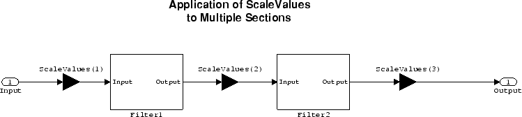
Signed
When you create a dfilt object for fixed-point filtering
(you set the property Arithmetic to
fixed, the property Signed
specifies whether the filter interprets coefficients as signed or unsigned. This
setting applies only to the coefficients. While the default setting is
true, meaning that all coefficients are assumed to be
signed, you can change the setting to false after you create
the fixed-point filter.
For example, create a fixed-point direct-form II transposed filter with both
negative and positive coefficients, and then change the property value for
Signed from true to
false to see what happens to the negative coefficient
values.
hd=dfilt.df2t(-5:5)

hd =

         FilterStructure: 'Direct-Form II Transposed'
              Arithmetic: 'double'
               Numerator: [-5 -4 -3 -2 -1 0 1 2 3 4 5]
             Denominator: 1
        PersistentMemory: false
                  States: [10x1 double]

set(hd,'arithmetic','fixed')
hd.numerator

ans =

    -5    -4    -3    -2    -1    0
     1     2     3     4     5

set(hd,'signed',false)
hd.numerator

ans =

     0     0     0     0     0     0
     1     2     3     4     5
Using unsigned coefficients limits you to using only positive coefficients in
your filter. Signed is a dynamic property — you
cannot set or change it until you switch the setting for the
Arithmetic property to fixed.
SosMatrix
When you convert a dfilt object to second-order section
form, or create a second-order section filter, sosMatrix
holds the filter coefficients as property values. Using the
double data type by default, the matrix is in [sections
coefficients per section] form, displayed as [15-x-6] for
filters with 6 coefficients per section and 15 sections, [15 6].
To demonstrate, the following code creates an order 30 filter using
second-order sections in the direct-form II transposed configuration. Notice the
sosMatrix property contains the coefficients for all
the sections.
d = fdesign.lowpass('n,fc',30,0.5);
hd = butter(d);

hd =

  FilterStructure: 'Direct-Form II, Second-Order Sections'
      Arithmetic: 'double'
       sosMatrix: [15x6 double]
     ScaleValues: [16x1 double]
PersistentMemory: false
          States: [2x15 double]

hd.arithmetic='fixed'

hd =

 FilterStructure: 'Direct-Form II, Second-Order Sections'
      Arithmetic: 'fixed'
       sosMatrix: [15x6 double]
     ScaleValues: [16x1 double]
PersistentMemory: false
                  States: [1x1 embedded.fi]

 CoeffWordLength: 16
  CoeffAutoScale: true
          Signed: true

 InputWordLength: 16
 InputFracLength: 15

  SectionInputWordLength: 16
   SectionInputAutoScale: true

 SectionOutputWordLength: 16
  SectionOutputAutoScale: true

        OutputWordLength: 16
              OutputMode: 'AvoidOverflow'

         StateWordLength: 16
         StateFracLength: 15

             ProductMode: 'FullPrecision'

         AccumWordLength: 40
           CastBeforeSum: true

               RoundMode: 'convergent'
            OverflowMode: 'wrap'

hd.sosMatrix

ans =

    1.0000    2.0000    1.0000    1.0000         0    0.9005
    1.0000    2.0000    1.0000    1.0000         0    0.7294
    1.0000    2.0000    1.0000    1.0000         0    0.5888
    1.0000    2.0000    1.0000    1.0000         0    0.4724
    1.0000    2.0000    1.0000    1.0000         0    0.3755
    1.0000    2.0000    1.0000    1.0000         0    0.2948
    1.0000    2.0000    1.0000    1.0000         0    0.2275
    1.0000    2.0000    1.0000    1.0000         0    0.1716
    1.0000    2.0000    1.0000    1.0000         0    0.1254
    1.0000    2.0000    1.0000    1.0000         0    0.0878
    1.0000    2.0000    1.0000    1.0000         0    0.0576
    1.0000    2.0000    1.0000    1.0000         0    0.0344
    1.0000    2.0000    1.0000    1.0000         0    0.0173
    1.0000    2.0000    1.0000    1.0000         0    0.0062
    1.0000    2.0000    1.0000    1.0000         0    0.0007
The SOS matrix is an M-by-6 matrix, where M is the number of sections in the
second-order section filter. Filter hd has M equal to 15 as
shown above (15 rows). Each row of the SOS matrix contains the numerator and
denominator coefficients (b's and a's) and the scale factors of the
corresponding section in the filter.
SectionInputAutoScale
Second-order section filters include this property that determines who the filter handles data in the transitions from one section to the next in the filter.
How the filter represents the data passing from one section to the next
depends on the property value of SectionInputAutoScale. The
representation the filter uses between the filter sections depends on whether
the value of SectionInputAutoScale is
true or false.
SectionInputAutoScale=truemeans the filter chooses the fraction length to maintain the value of the data between sections as close to the output values from the previous section as possible.trueis the default setting.SectionInputAutoScale=falseremoves the automatic scaling of the fraction length for the intersection data and exposes the property that controls the coefficient fraction length (SectionInputFracLength) so you can change it. For example, if the filter is a second-order, direct form FIR filter, settingSectionInputAutoScaletofalseexposes theSectionInputFracLengthproperty that specifies the fraction length applied to data between the sections.
SectionInputFracLength
Second-order section filters use quantizers at the input to each section of
the filter. The quantizers apply to the input data entering each filter section.
Note that the quantizers for each section are the same. To set the fraction
length for interpreting the input values, use the property value in
SectionInputFracLength.
In combination with CoeffWordLength,
SectionInputFracLength fully determines how the filter
interprets and uses the state values stored in the property
States. As with all word and fraction length
properties, SectionInputFracLength can be any integer,
including integers larger than CoeffWordLength, and positive
or negative integers. 15 bits is the default value when you create the filter
object.
SectionInputWordLength
SOS filters are composed of sections, each one a second-order filter.
Filtering data input to the filter involves passing the data through each filter
section. SectionInputWordLength specifies the word length
applied to data as it enters one filter section from the previous section. Only
second-order implementations of direct-form I transposed and direct-form II
transposed filters include this property.
The following diagram shows an SOS filter composed of sections (the bottom
part of the diagram) and a possible internal structure of each Section (the top
portion of the diagram), in this case — a direct form I transposed second
order sections filter structure. Note that the output of each section is fed
through a multiplier. If the gain of the multiplier =1, then
the last Cast block of the Section is ignored, and the format of the output is
NumSumQ.

SectionInputWordLength defaults to 16 bits.
SectionOutputAutoScale
Second-order section filters include this property that determines who the filter handles data in the transitions from one section to the next in the filter.
How the filter represents the data passing from one section to the next
depends on the property value of SectionOutputAutoScale.
The representation the filter uses between the filter sections depends on
whether the value of SectionOutputAutoScale is
true or false.
SectionOutputAutoScale=truemeans the filter chooses the fraction length to maintain the value of the data between sections as close to the output values from the previous section as possible.trueis the default setting.SectionOutputAutoScale=falseremoves the automatic scaling of the fraction length for the intersection data and exposes the property that controls the coefficient fraction length (SectionOutputFracLength) so you can change it. For example, if the filter is a second-order, direct form FIR filter, settingSectionOutputAutoScale=falseexposes theSectionOutputFracLengthproperty that specifies the fraction length applied to data between the sections.
SectionOutputFracLength
Second-order section filters use quantizers at the output from each section of
the filter. The quantizers apply to the output data leaving each filter section.
Note that the quantizers for each section are the same. To set the fraction
length for interpreting the output values, use the property value in
SectionOutputFracLength.
In combination with CoeffWordLength,
SectionOutputFracLength determines how the filter
interprets and uses the state values stored in the property
States. As with all fraction length properties,
SectionOutputFracLength can be any integer, including
integers larger than CoeffWordLength, and positive or
negative integers. 15 bits is the default value when you create the filter
object.
SectionOutputWordLength
SOS filters are composed of sections, each one a second-order filter.
Filtering data input to the filter involves passing the data through each filter
section. SectionOutputWordLength specifies the word length
applied to data as it leaves one filter section to go to the next. Only
second-order implementations direct-form I transposed and direct-form II
transposed filters include this property.
The following diagram shows an SOS filter composed of sections (the bottom
part of the diagram) and a possible internal structure of each Section (the top
portion of the diagram), in this case — a direct form I transposed second
order sections filter structure. Note that the output of each section is fed
through a multiplier. If the gain of the multiplier =1, then
the last Cast block of the Section is ignored, and the format of the output is
NumSumQ.
SectionOutputWordLength defaults to 16 bits.
StateAutoScale
Although all filters use states, some do not allow you to choose whether the filter automatically scales the state values to prevent overruns or bad arithmetic errors. You select either of the following settings:
StateAutoScale=truemeans the filter chooses the fraction length to maintain the value of the states as close to the double-precision values as possible. When you change the word length applied to the states (where allowed by the filter structure), the filter object changes the fraction length to try to accommodate the change.trueis the default setting.StateAutoScale=falseremoves the automatic scaling of the fraction length for the states and exposes the property that controls the coefficient fraction length so you can change it. For example, in a direct form I transposed SOS FIR filter, settingStateAutoScale=falseexposes theNumStateFracLengthandDenStateFracLengthproperties that specify the fraction length applied to states.
Each of the following filter structures provides the
StateAutoScale property:
df1tdf1tsosdf2tdf2tsosdffirt
Other filter structures do not include this property.
StateFracLength
Filter states stored in the property States have both
word length and fraction length. To set the fraction length for interpreting the
stored filter object state values, use the property value in
StateFracLength.
In combination with CoeffWordLength,
StateFracLength fully determines how the filter
interprets and uses the state values stored in the property
States.
As with all fraction length properties, StateFracLength
can be any integer, including integers larger than
CoeffWordLength, and positive or negative integers. 15
bits is the default value when you create the filter object.
States
Digital filters are dynamic systems. The behavior of dynamic systems (their response) depends on the input (stimulus) to the system and the current or previous state of the system. You can say the system has memory or inertia. All fixed- or floating-point digital filters (as well as analog filters) have states.
Filters use the states to compute the filter output for each input sample, as well using them while filtering in loops to maintain the filter state between loop iterations. This toolbox assumes zero-valued initial conditions (the dynamic system is at rest) by default when you filter the first input sample. Assuming the states are zero initially does not mean the states are not used; they are, but arithmetically they do not have any effect.
Filter objects store the state values in the property
States. The number of stored states depends on the
filter implementation, since the states represent the delays in the filter
implementation.
When you review the display for a filter object with fixed arithmetic, notice
that the states return an embedded fi object, as you see
here.
b = ellip(6,3,50,300/500);
hd=dfilt.dffir(b)

hd =

         FilterStructure: 'Direct-Form FIR'
              Arithmetic: 'double'
               Numerator: [0.0773 0.2938 0.5858 0.7239 0.5858 0.2938 0.0773]
        PersistentMemory: false
                  States: [6x1 double]


hd.arithmetic='fixed'

hd =

         FilterStructure: 'Direct-Form FIR'
              Arithmetic: 'fixed'
               Numerator: [0.0773 0.2938 0.5858 0.7239 0.5858 0.2938 0.0773]
        PersistentMemory: false
                  States: [1x1 embedded.fi]

         CoeffWordLength: 16
          CoeffAutoScale: 'on'
                  Signed: 'on'

         InputWordLength: 16
         InputFracLength: 15

        OutputWordLength: 16
              OutputMode: 'AvoidOverflow'

             ProductMode: 'FullPrecision'

         AccumWordLength: 40
           CastBeforeSum: 'on'

               RoundMode: 'convergent'
            OverflowMode: 'wrap'

         InheritSettings: 'off'
fi objects provide fixed-point support for the filters. To
learn more about the details about fi objects, refer to your
Fixed-Point Designer documentation.
The property States lets you use a fi
object to define how the filter interprets the filter states. For example, you
can create a fi object in MATLAB, then assign the object to States, as follows:
statefi=fi([],16,12)

statefi =

[]
   DataTypeMode = Fixed-point: binary point scaling
         Signed = true
    Wordlength = 16
Fractionlength = 12
This fi object does not have a value associated (notice the
[] input argument to fi for the
value), and it has word length of 16 bits and fraction length of 12 bit. Now you
can apply statefi to the States property
of the filter hd.
set(hd,'States',statefi);
Warning: The 'States' property will be reset to the value
specified at construction before filtering.
Set the 'PersistentMemory' flag to 'True'
to avoid changing this property value.
hd

hd =

         FilterStructure: 'Direct-Form FIR'
              Arithmetic: 'fixed'
               Numerator: [0.0773 0.2938 0.5858 0.7239 0.5858
                           0.2938 0.0773]
        PersistentMemory: false
                  States: [1x1 embedded.fi]

         CoeffWordLength: 16
          CoeffAutoScale: 'on'
                  Signed: 'on'

         InputWordLength: 16
         InputFracLength: 15

        OutputWordLength: 16
              OutputMode: 'AvoidOverflow'

             ProductMode: 'FullPrecision'
         AccumWordLength: 40
           CastBeforeSum: 'on'

               RoundMode: 'convergent'
            OverflowMode: 'wrap'
StateWordLength
While all filters use states, some do not allow you to directly change the
state representation — the word length and fraction lengths —
independently. For the others, StateWordLength specifies
the word length, in bits, the filter uses to represent the states. Filters that
do not provide direct state word length control include:
df1dfasymfirdffirdfsymfir
For these structures, the filter derives the state format from the input
format you choose for the filter — except for the df1
IIR filter. In this case, the numerator state format comes from the input format
and the denominator state format comes from the output format. All other filter
structures provide control of the state format directly.
TapSumFracLength
Direct-form FIR filter objects, both symmetric and antisymmetric, use this
property. To set the fraction length for output from the sum operations that
involve the filter tap weights, use the property value in
TapSumFracLength. To enable this property, set the
TapSumMode to SpecifyPrecision in
your filter.
As you can see in this code example that creates a fixed-point asymmetric FIR
filter, the TapSumFracLength property becomes available
after you change the TapSumMode property value.
hd=dfilt.dfasymfir

hd =

         FilterStructure: 'Direct-Form Antisymmetric FIR'
              Arithmetic: 'double'
               Numerator: 1
        PersistentMemory: false
                  States: [0x1 double]

set(hd,'arithmetic','fixed');
hd

hd =

         FilterStructure: 'Direct-Form Antisymmetric FIR'
              Arithmetic: 'fixed'
               Numerator: 1
        PersistentMemory: false
                  States: [1x1 embedded.fi]

         CoeffWordLength: 16
          CoeffAutoScale: true
                  Signed: true

         InputWordLength: 16
         InputFracLength: 15

        OutputWordLength: 16
              OutputMode: 'AvoidOverflow'

              TapSumMode: 'KeepMSB'
        TapSumWordLength: 17

             ProductMode: 'FullPrecision'

         AccumWordLength: 40

           CastBeforeSum: true
               RoundMode: 'convergent'
            OverflowMode: 'wrap'
With the filter now in fixed-point mode, you can change the
TapSumMode property value to
SpecifyPrecision, which gives you access to the
TapSumFracLength property.
set(hd,'TapSumMode','SpecifyPrecision');
hd

hd =

         FilterStructure: 'Direct-Form Antisymmetric FIR'
              Arithmetic: 'fixed'
               Numerator: 1
        PersistentMemory: false
                  States: [1x1 embedded.fi]

         CoeffWordLength: 16
          CoeffAutoScale: true
                  Signed: true

         InputWordLength: 16
         InputFracLength: 15

        OutputWordLength: 16
              OutputMode: 'AvoidOverflow'

              TapSumMode: 'SpecifyPrecision'
        TapSumWordLength: 17
        TapSumFracLength: 15

             ProductMode: 'FullPrecision'

         AccumWordLength: 40

           CastBeforeSum: true
               RoundMode: 'convergent'
            OverflowMode: 'wrap'
In combination with TapSumWordLength,
TapSumFracLength fully determines how the filter
interprets and uses the state values stored in the property
States.
As with all fraction length properties, TapSumFracLength
can be any integer, including integers larger than
TapSumWordLength, and positive or negative integers. 15
bits is the default value when you create the filter object.
TapSumMode
This property, available only after your filter is in fixed-point mode,
specifies how the filter outputs the results of summation operations that
involve the filter tap weights. Only symmetric (dfilt.dfsymfir) and
antisymmetric (dfilt.dfasymfir) FIR filters use
this property.
When available, you select from one of the following values:
FullPrecision— means the filter automatically chooses the word length and fraction length to represent the results of the sum operation so they retain all of the precision provided by the inputs (addends).KeepMSB— means you specify the word length for representing tap sum summation results to keep the higher order bits in the data. The filter sets the fraction length to discard the LSBs from the sum operation. This is the default property value.KeepLSB— means you specify the word length for representing tap sum summation results to keep the lower order bits in the data. The filter sets the fraction length to discard the MSBs from the sum operation. Compare to theKeepMSBoption.SpecifyPrecision— means you specify the word and fraction lengths to apply to data output from the tap sum operations.
TapSumWordLength
Specifies the word length the filter uses to represent the output from tap sum
operations. The default value is 17 bits. Only dfasymfir and
dfsymfir filters include this property.