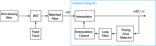
The symbol timing synchronizer algorithm is based on a phased lock loop (PLL) algorithm that consists of four components:

For OQPSK modulation, the in-phase and quadrature signal components are first aligned (as in QPSK modulation) using a state buffer to cache the last half symbol of the previous input. After initial alignment, the remaining synchronization process is the same as for QPSK modulation.

This block diagram shows an example of a timing synchronizer. In the figure, the symbol timing PLL operates on x(t), the received sample signal after matched filtering. The symbol timing PLL outputs the symbol signal, $$x(k{T}_{\text{s}}+\widehat{\tau })$$, after correcting for the clock skew between the transmitter and receiver.

The symbol timing synchronizer supports non-data-aided TED and decision-directed TED methods. This table shows the timing estimate expressions for the TED method options.

Non-data-aided TED uses received samples without any knowledge of the transmitted signal or the results of the channel estimation. Non-data-aided TED is used to estimate the timing error for signals with modulation schemes that have constellation points aligned with the in-phase or quadrature axis. Examples of signals suitable for the Gardner or early-late methods include QPSK-modulated signals with a zero phase offset that has points at {1+0i, 0+1i, -1+0i, 0−1i} and BPSK-modulated signals with a zero phase offset.

The early-late method is similar to the Gardner method. The Gardner method performs better in systems with high SNR values because it has lower self noise than the early-late method.

Decision-directed TED uses the sign function to estimate the in-phase and quadrature components of received samples, which result in lower computational complexity than non-data-aided TED.

Because the decision-directed methods (zero-crossing and Mueller-Muller) estimate timing error based on the sign of the in-phase and quadrature components of signals passed to the synchronizer, they are not recommended for constellations that have points with either a zero in-phase or a quadrature component. $$x(k{T}_{\text{s}}+\widehat{\tau })$$ and $$y(k{T}_{\text{s}}+\widehat{\tau })$$ are the in-phase and quadrature components of the input signals to the timing error detector, where $$\widehat{\tau }$$ is the estimated timing error. The Mueller-Muller method coefficients $${\widehat{a}}_0(k)$$ and $${\widehat{a}}_1(k)$$ are the estimates of $$x(k{T}_{\text{s}}+\widehat{\tau })$$ and $$y(k{T}_{\text{s}}+\widehat{\tau })$$. The timing estimates are made by applying the sign function to the in-phase and quadrature components and are used for only the decision-directed TED methods.

The time delay is estimated from the fixed-rate samples of the matched filter, which are asynchronous with the symbol rate. Because the resulting samples are not aligned with the symbol boundaries, an interpolator is used to "move" the samples. Because the time delay is unknown, the interpolator must be adaptive. Moreover, because the interpolant is a linear combination of the available samples, it can be thought of as the output of a filter.

The interpolator uses a piecewise parabolic interpolator with a Farrow structure and coefficient α set to 1/2 (see Rice, Michael, Digital Communications: A Discrete-Time Approach).

Interpolation control provides the interpolator with the basepoint index and fractional interval. The basepoint index is the sample index nearest to the interpolant. The fractional interval is the ratio of the time between the interpolant and its basepoint index and the interpolation interval.

Interpolation is performed for every sample, and a strobe signal is used to determine if the interpolant is output. The synchronizer uses a modulo-1 counter interpolation control to provide the strobe and the fractional interval for use with the interpolator.

The synchronizer uses a proportional-plus integrator (PI) loop filter. The proportional gain, K₁, and the integrator gain, K₂, are calculated by

and

The interim term, θ, is given by

where: