orthfilt

Orthogonal wavelet filter set

Syntax

[Lo_D,Hi_D,Lo_R,Hi_R] = orthfilt(W)

Description

[Lo_D,Hi_D,Lo_R,Hi_R] = orthfilt(W) computes the four filters associated with the scaling filter W corresponding to a wavelet:

`Lo_D`	Decomposition low-pass filter
`Hi_D`	Decomposition high-pass filter
`Lo_R`	Reconstruction low-pass filter
`Hi_R`	Reconstruction high-pass filter

For an orthogonal wavelet, in the multiresolution framework, we start with the scaling function ϕ and the wavelet function ψ. One of the fundamental relations is the twin-scale relation:

$\frac{1}{2} ϕ (\frac{x}{2}) = \sum_{n \in Z} w_{n} ϕ (x - n)$

All the filters used in dwt and idwt are intimately related to the sequence ${(w_{n})}_{n \in Z}$ . Clearly if ϕ is compactly supported, the sequence (w_n) is finite and can be viewed as a FIR filter. The scaling filter W is

A low-pass FIR filter
Of length 2N
Of sum 1
Of norm

For example, for the db3 scaling filter,

load db3 
db3
db3 =
    0.2352 0.5706 0.3252 -0.0955 -0.0604 0.0249

sum(db3)
ans =
    1.000
    norm(db3)
ans =
    0.7071

From filter W, we define four FIR filters, of length 2N and norm 1, organized as follows:

Filters	Low-Pass	High-Pass
Decomposition	`Lo_D`	`Hi_D`
Reconstruction	`Lo_R`	`Hi_R`

The four filters are computed using the following scheme:

where qmf is such that Hi_R and Lo_R are quadrature mirror filters (i.e., Hi_R(k) = (-1)^kLo_R(2N + 1 - k), for k = 1, 2, Ä, 2N), and where wrev flips the filter coefficients. So Hi_D and Lo_D are also quadrature mirror filters. The computation of these filters is performed using orthfilt.

Examples

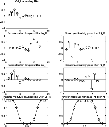
% Load scaling filter. 
load db8; w = db8; 
subplot(421); stem(w); 
title('Original scaling filter');

% Compute the four filters. 
[Lo_D,Hi_D,Lo_R,Hi_R] = orthfilt(w); 
subplot(423); stem(Lo_D); 
title('Decomposition low-pass filter'); 
subplot(424); stem(Hi_D); 
title('Decomposition high-pass filter'); 
subplot(425); stem(Lo_R); 
title('Reconstruction low-pass filter'); 
subplot(426); stem(Hi_R); 
title('Reconstruction high-pass filter');

% Check for orthonormality. 
df = [Lo_D;Hi_D];
rf = [Lo_R;Hi_R];
id = df*df'

id =
    1.0000         0
         0    1.0000

id = rf*rf'

id =
    1.0000         0
         0    1.0000

% Check for orthogonality by dyadic translation, for example:
df = [Lo_D 0 0;Hi_D 0 0]; 
dft = [0 0 Lo_D; 0 0 Hi_D]; 
zer = df*dft'

zer =

    1.0e-12 *
    -0.1883 0.0000
    -0.0000 -0.1883

% High- and low-frequency illustration. 
fftld = fft(Lo_D); ffthd = fft(Hi_D); 
freq = [1:length(Lo_D)]/length(Lo_D); 
subplot(427); plot(freq,abs(fftld)); 
title('Transfer modulus: low-pass');
subplot(428); plot(freq,abs(ffthd)); 
title('Transfer modulus: high-pass')
% Editing some graphical properties,
% the following figure is generated.

References

Daubechies, I. (1992), Ten lectures on wavelets, CBMS-NSF conference series in applied mathematics, SIAM Ed. pp. 117–119, 137, 152.

Documentation

orthfilt

Syntax

Description

Examples

References

See Also

Wavelet Toolbox Documentation

Support