Managing Estimation Speed and Memory

Ways to Speed up Frequency Response Estimation

The most time consuming operation during frequency response estimation is the simulation of your Simulink^® model. You can try to speed up the estimation using any of the following ways:

Reducing simulation stop time
Specifying accelerator mode
Using parallel computing

Reducing Simulation Stop Time

The time it takes to perform frequency response estimation depends on the simulation stop time.

To obtain the simulation stop time, in the Model Linearizer, in the Linear Analysis Workspace, select the input signal. The simulation time will be displayed in the Variable Preview.

To obtain the simulation stop time from the input signal using MATLAB^® Code:

tfinal = getSimulationTime(input)

where input is the input signal. The simulation stop time, tfinal, serves as an indicator of the frequency response estimation duration.

You can reduce the simulation time by modifying your signal properties.

Input Signal	Action	Caution
Sinestream	Decrease the number of periods per frequency, `NumPeriods`, especially at lower frequencies.	You model must be at steady state to achieve accurate frequency response estimation. Reducing the number of periods might not excite your model long enough to reach steady state.
Chirp	Decrease the signal sample time, `Ts`, or the number of samples, `NumSamples`.	The frequency resolution of the estimated response depends on the number of samples `NumSamples`. Decreasing the number of samples decreases the frequency resolution of the estimated frequency response.

For information about modifying input signals, see Modify Estimation Input Signals.

Specifying Accelerator Mode

You can try to speed up frequency response estimation by specifying the Rapid Accelerator or Accelerator mode in Simulink.

For more information, see What Is Acceleration?.

Using Parallel Computing

You can try to speed up frequency response estimation using parallel computing in the following situations:

Your model has multiple inputs.
Your single-input model uses a sinestream input signal, where the sinestream SimulationOrder property has the value 'OneAtATime'.
For information on setting this option, see the frest.Sinestream reference page.

In these situations, frequency response estimation performs multiple simulations. If you have installed the Parallel Computing Toolbox™ software, you can run these multiple simulations in parallel on multiple MATLAB sessions (pool of MATLAB workers).

For more information about using parallel computing, see Speeding Up Estimation Using Parallel Computing.

Speeding Up Estimation Using Parallel Computing

Configuring MATLAB for Parallel Computing

You can use parallel computing to speed up a frequency response estimation that performs multiple simulations. You can use parallel computing with the Model Linearizer and frestimate. When you perform frequency response estimation using parallel computing, the software uses the available parallel pool. If no parallel pool is available and Automatically create a parallel pool is selected in your Parallel Computing Toolbox preferences, then the software starts a parallel pool using the settings in those preferences.

You can configure the software to automatically detect model dependencies and temporarily add them to the parallel pool workers. However, to ensure that workers are able to access the undetected file and path dependencies, create a cluster profile that specifies the same. The parallel pool used to optimize the model must be associated with this cluster profile. For information on creating a cluster profile, see Add and Modify Cluster Profiles (Parallel Computing Toolbox).

To manually open a parallel pool that uses a specific cluster profile, use:

parpool(MyProfile)

MyProfile is the name of a cluster profile.

Estimating Frequency Response Using Parallel Computing Using Model Linearizer

After you configure your parallel computing settings, as described in Configuring MATLAB for Parallel Computing, you can estimate the frequency response of a Simulink model using the Model Linearizer.

In the Model Linearizer, in the Estimation tab, click More Options.
This action opens the Options for frequency response estimation dialog box.
In the Parallel Options tab, select the Use the parallel pool during estimation check box.
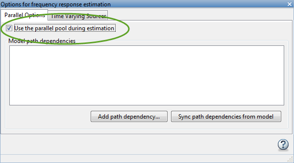
(Optional) Click Add path dependency.
The Browse For Folder dialog box opens. Navigate and select the directory to add to the model path dependencies.
Click OK.

Tip
Alternatively, manually specify the paths in the Model path dependencies list. You can specify the paths separated with a new line.
(Optional) Click Sync path dependencies from model.
This action finds the model path dependencies in your Simulink model and adds them to the Model path dependencies list box.

Estimating Frequency Response Using Parallel Computing (MATLAB Code)

After you configure your parallel computing settings, as described in Configuring MATLAB for Parallel Computing, you can estimate the frequency response of a Simulink model.

Find the paths to files that your Simulink model requires to run, called path dependencies.
```
dirs = frest.findDepend(model)
```
dirs is a cell array of character vectors containing path dependencies, such as referenced models, data files, and S-functions.
For more information about this command, see frest.findDepend.
To learn more about model dependencies, see Analyze Model Dependencies and Dependency Analyzer Scope and Limitations.
(Optional) Check that dirs includes all path dependencies. Append any missing paths to dirs:
```
dirs = vertcat(dirs,'\\hostname\C$\matlab\work')
```
(Optional) Check that all workers have access to the paths in dirs.
If any of the paths resides on your local drive, specify that all workers can access your local drive. For example, this command converts all references to the C drive to an equivalent network address that is accessible to all workers:
```
dirs = regexprep(dirs,'C:/','\\\\hostname\\C$\\')
```
Enable parallel computing and specify model path dependencies by creating an options object using the frestimateOptions command:
```
options = frestimateOptions('UseParallel','on','ParallelPathDependencies',dirs)
```
Tip
To enable parallel computing for all estimations, select the global preference Use the parallel pool when you use the "frestimate" command check box in the MATLAB preferences. If your model has path dependencies, you must create your own frequency response options object that specifies the path dependencies before beginning estimation.

Estimate the frequency response:

[sysest,simout] = frestimate('model',io,input,options)

For an example of using parallel computing to speed up estimation, see Speed Up Frequency Response Estimation Using Parallel Computing.

Managing Memory During Frequency Response Estimation

Frequency response estimation terminates when the simulation data exceed available memory. Insufficient memory occurs in the following situations:

Your model performs data logging during a long simulation. A sinestream input signal with four periods at a frequency of 1e-3 rad/s runs a Simulink simulation for 25,000 s. If you are logging signals using To Workspace blocks, this length of simulation time might cause memory problems.
A model with an output point discrete sample time of 1e-8 s that simulates at 5-Hz frequency (0.2 s of simulation per period), results in $\frac{0.2}{1 e - 8} = 2$ million samples of data per period. Typically, this amount of data requires over 300 MB of storage.

To avoid memory issues while estimating frequency response:

Disable any signal logging in your Simulink model.
To learn how you can identify which model components log signals and disable signal logging, see Signal Logging.
Try one or more of the actions listed in the following sections:
- Model-Specific Ways to Avoid Memory Issues
- Input-Signal-Specific Ways to Avoid Memory Issues
Repeat the estimation.

Model-Specific Ways to Avoid Memory Issues

To avoid memory issues, try one or more of the actions listed in the following table, as appropriate for your model type.

Model Type	Action
Models with fast discrete sample time specified at output point	Insert a Rate Transition block at the output point to lower the sample rate, which decreases the amount of logged data. Move the linearization output point to the output of the Rate Transition block before you estimate. Ensure that the location of the original output point does not have aliasing as a result of rate conversion. For information on determining sample rate, see View Sample Time Information. If your estimation is slow, see Ways to Speed up Frequency Response Estimation.
Models with multiple input and output points (MIMO models)	Estimate the response for all input/output combinations separately. Then, combine the results into one MIMO model using the data format described in Create Frequency-Response Model from Data. Use parallel computing to run the independent simulations in parallel on different computers. See Speeding Up Estimation Using Parallel Computing.

Model Type

Action

Models with fast discrete sample time specified at output point

Insert a Rate Transition block at the output point to lower the sample rate, which decreases the amount of logged data. Move the linearization output point to the output of the Rate Transition block before you estimate. Ensure that the location of the original output point does not have aliasing as a result of rate conversion.

For information on determining sample rate, see View Sample Time Information. If your estimation is slow, see Ways to Speed up Frequency Response Estimation.

Models with multiple input and output points (MIMO models)

Estimate the response for all input/output combinations separately. Then, combine the results into one MIMO model using the data format described in Create Frequency-Response Model from Data.
Use parallel computing to run the independent simulations in parallel on different computers. See Speeding Up Estimation Using Parallel Computing.

Input-Signal-Specific Ways to Avoid Memory Issues

To avoid memory issues, try one or more of the actions listed in the following table, as appropriate for your input signal type.

Input Signal Type	Action
Sinestream	Remove low frequencies from your input signal for which you do not need the frequency response. Modify the sinestream signal to estimate each frequency separately by setting the `SimulationOrder` option to `OneAtATime`. Then estimate using a `frestimate` syntax that does not request the simulated time-response output data, for example `sysest = frestimate(model,io,input)`. Use parallel computing to run independent simulations in parallel on different computers. See Speeding Up Estimation Using Parallel Computing. Divide the input signal into multiple signals using `fselect`. Estimate the frequency response for each signal separately using `frestimate`. Then, combine results using `fcat`.
Chirp	Create separate input signals that divide up the swept frequency range of the original signal into smaller sections using `frest.Chirp`. Estimate the frequency response for each signal separately using `frestimate`. Then, combine results using `fcat`.
Random	Decrease the number of samples in the random input signal by changing `NumSamples` before estimating. See Time Response Is Noisy.

Documentation