Configuration
Define system simulation settings
- Library:
RF Blockset / Circuit Envelope / Utilities

Description
Use the Configuration block to set the model conditions for a circuit envelope simulation. The block parameter defines RF and solver attributes. The RF attributes include properties such as simulation frequencies, harmonic order, envelope bandwidth, and thermal noise. The solver attributes include transient analysis types, tolerances, and small signal approximation.
The small signal transient simulation performs a full non-linear harmonic balance steady state solution to determine an operation point for a subsequent linear transient analysis. This option allows you to capture the right spectral behavior of a small signal affected by large constant (over carrier) signals.
Connect one Configuration block to each topologically distinct RF Blockset™ subsystem. Each Configuration block defines the parameters of the
connected RF Blockset subsystem. To see an example of the Configuration block in a model, enter
RFNoiseExample in the MATLAB Command Window.
For an introduction to RF simulation, see Simulate High Frequency Components.
Parameters
Automatically select fundamental tones and harmonic order — Automatically select fundamental tones and harmonic order
on (default) | off
Select this parameter to choose Fundamental tones and Harmonic order parameters automatically when you update the model. Automatic selection does not always return the smallest possible set of simulation frequencies. This approach uses conservative number of simulation frequencies to capture the non -linear behavior of the system.
To set the Fundamental tones and Harmonic order, clear this parameter. A smaller set of simulation frequencies decreases simulation time and decreases memory requirements. However, a decrease in simulation frequencies can reduce accuracy.
Fundamental tones — Fundamental tones of set of simulation frequency
vector of positive integers in Hz
Fundamental tones of a set of simulation frequencies, specified as a vector of positive integers in Hz.
Dependencies
To enable this parameter, clear Automatically select fundamental tones and harmonic order.
Harmonic order — Harmonic order for each fundamental tone
vector of positive integers
Harmonic order for each fundamental tone, specified as a vector of positive integer. You can also specify a scalar and this value is applied to each Fundamental tones.
Dependencies
To enable this parameter, clear Automatically select fundamental tones and harmonic order.
Total simulation frequencies: Computed at simulation time — Displays number for simulation frequencies
button
The block determines the simulation frequencies based on the fundamental tones and their respective harmonic order. The solver computes a solution to the network at each simulation frequency and the computation time scales according to the total number of simulation frequencies.
Combinations of fundamental tones determine the set of simulation frequencies: [m*f1 + n*f2 + …]. In this case, the fundamental tones are represented by [fs1,f2,…], and the integers m and n are integers bounded by the corresponding Harmonic order, |m| ≦h1, |n| ≦h2, etc. Only positive frequencies are considered.
Click View to open the dialog box containing additional
information about the simulation frequencies in your system. The
Configuration block displays the number of simulation frequencies
for a nonlinear model. For linear models, the actual number of frequencies are
automatically optimized during simulation.
By clicking a listed simulation frequency, you can see which linear or multiple combinations of fundamental tones represent that frequency. From the dialog box, you can also plot the simulation frequencies on a number line.
Consider a single fundamental tone f1 = 2 GHz and
corresponding harmonic order h1 = 3. The set of
simulation frequencies are: [0, f1, 2f1, 3f1] = [0GHz, 2 GHz, 4 GHz,
6GHz].
Consider a circuit with two fundamental tones [f1 = 2 GHz, f2 = 50
MHz] and corresponding harmonic orders h1 = h2 = 1. This
setup results in five simulation frequencies with values: [0, f2, f1-f2, f1,
f1+f2].
Consider a circuit with two fundamental tones [f1 = 2 GHz, f2 =
3GHz] and corresponding harmonic orders h1 = 1, and
h2 = 3. This setup results in 11 simulation frequencies with
values: [0, f2, f1-f2, f1, f1+f2, -f1+2f2, 2f2, -f1+3f2, f1+2f2, 3f2,
f1+3f2].
The set of simulation frequencies must include all carrier frequencies specified in the RF Blockset subsystem such as the carrier frequencies inside Inport, Outport, and source blocks.
Dependencies
To enable this parameter, select Automatically select fundamental tones and harmonic order. If you clear Automatically select fundamental tones and harmonic order, the option becomes, Total simulation frequencies: N/A: Fundamental tones undefined.
Step size — Time step for fixed step solver configuration
1e-6 (default) | scalar in seconds
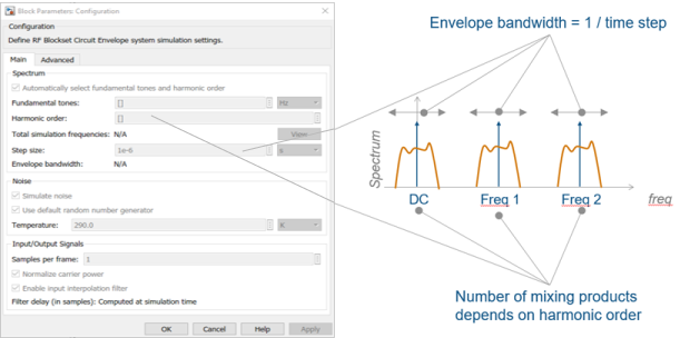
Time step for fixed step solver configuration, specified as a scalar in seconds. The inverse of the time step determines the simulation bandwidth of the signal envelope centered around each simulation frequency.
The time step of a circuit envelope simulation should be commensurate to relative signal bandwidth and not to the absolute value of the carrier frequency.
The default (1e-6s) is sufficient for modelling envelope signals with bandwidths of up to 1/h, or 1MHz. Simulation accuracy is reduced when simulating close to the maximum bandwidth. Reduce the step size to model signals with a larger bandwidth, or improve accuracy.
The simulation speed is inversely proportional to the simulation step size. A smaller simulation step size corresponds to a wider envelope bandwidth and to a slower simulation.
When the white noise is simulated, the noise bandwidth for each simulation frequency is equal to 1/h.
Envelope bandwidth — Maximum simulated envelope bandwidth
1 MHz (default) | scalar in Hz
Maximum simulated envelope bandwidth, returned as a scalar in Hz. Configuration block automatically calculates this value using the Step size parameter. The formula used is: .
Simulate noise — Globally enable or disable noise modeling
on (default) | off
Select this parameter to globally enable noise modeling in RF Blockset circuits. When this check box is selected:
Amplifier and Mixer blocks use the value of their respective Noise figure (dB) parameters.
Amplifier and Mixer blocks simulate with thermal noise at the temperature specified by the Temperature parameter.
Resistor blocks model thermal noise using the Temperature parameters.
Noise blocks model a specified noise power as a voltage or current source.
To disable noise modeling globally, clear this parameter.
Use default random number generator — Default pseudorandom noise stream for RF Blockset sources
on (default) | off
Select this parameter to retain the default pseudo random noise stream for RF Blockset sources. Clear this option to specify an independent pseudo random number stream for the RF Blockset topological subsystem and determine the seed of the noise stream.
Dependencies
To expose this parameter, select Simulate noise.
Noise seed — Seed of the independent pseudo random number stream
0 (default) | scalar positive integer
Seed of the independent pseudo random number stream, specified as a scalar positive integer.
Dependencies
To expose this parameter, clear Use default random number generator.
Temperature — Global noise temperature
290.0K | scalar integer in kelvin
Global noise temperature, specified as a scalar integer in kelvin.
Samples per frame — Number of samples in each channel of input signal to Inport block
1 | positive scalar integer
Number of samples in each channel of input signal to Inport block, specified as a positive scalar integer less than or equal to
1024. A channel corresponds to an input frequency in the Inport
block.
Note
The recommended maximum number of samples per frame are 1024.
Normalize Carrier Power — Normalize power of carrier signal
on (default) | off
Select this option to normalize the carrier power such that the average power of the signal is:
In this case, the equation gives the corresponding passband signal at ω:
where:
I(t) is the in-phase part of the carrier signal.
Q(t) is the quadrature part of the carrier signal.
fk are the carrier frequencies.
Clear this option so the average power of the carrier signal is:
In this case, the corresponding passband signal at ω represented by the equation
0 carrier frequency is a special case. Its passband representation is always I and average power I2
Enable input interpolation filter — Automatic interpolation of lower rate baseband signal to higher rate RF signal
on (default) | off
Select this option to enable input interpolation filter to up sample the input signal rates to fit sample rate of the RF solver. You can now directly use baseband communication signals using a lower sample rate in a wider band circuit. This filter introduces a delay in the RF signal. Filter delay (in samples) shows the delay introduced after you simulate the model.
Note
When you enable this filter,
The RF-to-baseband sample rate ratio must be 2, 4, 6, or 8.
The RF Blockset model can have only one Inport block.
Transient analysis — Fixed-step solver of RF Blockset environment
Auto (default) | NDF2 | Trapezoidal Rule | Backward Euler
Fixed-step solver of RF Blockset environment, specified as one of the following:
Auto: Set this parameter toAuto, when you are not sure which solver to use.NDF2: Set this parameter toNDF2to balance narrowband and wideband accuracy. This solver is suitable for situations where the frequency content of the signals in the system is unknown relative to the Nyquist rate.Trapezoidal Rule: Set this parameter toTrapezoidal Rulefor narrowband simulations. Frequency warping and the lack of damping effects make this method inappropriate for most wideband simulations.Backward Euler: Set this parameter toBackward Eulerto simulate the largest class of systems and signals. Damping effects make this solver suitable for wideband simulation, but overall accuracy is low.
The RF Blockset solver is an extension of the Simscape™ local solver. For more information on the Simscape local solver, see the Solver Configuration block reference page.
Approximate transient as small signal — Choose small subset of frequencies for transient small signal analysis
off (default) | on
Select this option to choose a small subset of frequencies for transient small signal analysis.
Use all steady-state simulation frequencies for small signal analysis — Choose all steady-state simulation frequencies
on (default) | off
Select this option to choose all steady-state simulation frequencies. Clear this option to specify the frequencies for small signal transient simulation.
Dependencies
To expose this parameter, check Approximate transient as small signal.
Small signal frequencies — Frequencies for small signal transient simulation
scalar | vector
Frequencies for small signal transient simulation, specified as a scalar or vector. The frequencies specified are contained in the entire set of simulation frequencies determined from Fundamental tones and Harmonic order in the Main tab.
The default values in this box and the corresponding units are not constants. The values depend on the state of the configuration dialog box when Use all steady-state simulation frequencies for small signal analysis is first cleared.
Dependencies
To expose this parameter, clear Use all steady-state simulation frequencies for small signal analysis.
Populate Frequencies — Tool to choose small signal transient frequencies
button
Tool to choose small signal transient frequencies to populate Small signal frequencies. The selected frequencies are a subset of the simulation frequencies determined from Fundamental tones and Harmonic order inputs in the Main tab. The entire set of simulation frequencies are given in the combo box on the right-hand side of the dialog box and the selected frequencies are highlighted. You can select by directly choosing the frequencies in the selection box, or by choosing the desired tones and harmonic order in the Small signal selection panel and pressing Select. The Tones(Hz) and Harmonic order values in the combo boxes are also populated using Fundamental tones and Harmonic order inputs in the Main tab.

Dependencies
To expose this parameter, clear Use all steady-state simulation frequencies for small signal analysis.
Relative tolerance — Relative newton tolerance for system variables
1e-3 (default) | real positive finite scalar
Relative newton tolerance for system variables, specified as a real positive finite scalar.
Absolute tolerance — Absolute newton tolerance for system variables
1e-6 (default) | real positive finite scalar
Absolute newton tolerance for system variables, specified as a real positive finite scalar.
Maximum iterations — Number iterations required for convergence
10 (default) | real positive integer scalar
Number iterations required for convergence, specified as a real positive integer scalar.
Error estimation — Check for error of convergence in system variables
2-norm over all variables (default) | Each variable separately
Check for error of convergence in system variables, specified as:
2-norm over all variables: Use this option to calculate the 2-norm of all the state variables and then check the error in convergence of state variables.Each variable separately: Use this option to check the error in convergence of each variable separately.
Restore Default Settings — Restore newton solver to default values
button
Restore newton solver to default values, specified as a button.
Model Examples


More About
Simulation Setup and Complexity
The key parameters in setting up a Circuit Envelope simulation are the fundamental tones, the harmonic order, and the step size. To speed up simulation, you can trade off the simulation step size and the total number of simulation frequencies.
For example, suppose that you have two large inputs signals each with 100 MHz bandwidth, centered around 10 GHz, and 10.1 GHz respectively. You can simulate the two signals using two separate fundamental tones [10 10.1] GHz. Each tone has a harmonic order of 3 (for a total of 25 simulation frequencies), and a simulation step size equal to 1/200MHz = 5 ns.
You could also set up the RF subsystem so that both of the signals are within the same simulation bandwidth centered around 10.05 GHz. In this case, you set the harmonic order equal to 3 (for a total of 4 simulation frequencies), and a simulation step size equal to 1/400MHz = 2.5 ns. The latter configuration is faster as the number of simulation frequencies is smaller by a factor 3, and the simulation step size is only smaller by a factor 2.
When setting up a circuit envelope simulation, avoid overlapping envelopes. The thermal noise generated by passive components are accounted for separately in each subband thus allowing for overlap of separate envelopes.
Criteria for Determining Simulation Step Size
The simulation step size must be small enough to capture the signal bandwidth and in-band spectral regrowth.
For example, your complex input Simulink signal has a sample frequency equal to 10 MHz. The minimum time step required to simulate this signal is 1/20 MHz = 50 ns. You can use an oversampling factor from 4 through 8, corresponding to a simulation time step between 25 ns and 12.5 ns. This captures the spectral regrowth caused by non-linear effects.
By default, the configuration block allows automatic interpolation of lower rate baseband signal to higher rate RF signal. If you disable this property, it is recommended that you use the same step size as the input Simulink signals. The input port resamples the input signal with the step size specified in the Configuration block. Using the same step size avoids undesired aliasing effects. It is best to resample the Simulink signals before importing them in RF Blockset using either analog (continuous time) or digital (discrete time) interpolation filters.
