dsp.Crosscorrelator

Cross-correlation of two inputs

Description

The dsp.Crosscorrelator System object™ computes the cross-correlation of two N-D input arrays along the first dimension. The computation can be done in the time domain or frequency domain. You can specify the domain through the Method property. In the time domain, the object convolves the first input signal, u, with the time-reversed complex conjugate of the second input signal, v. To compute the cross-correlation in the frequency domain, the object:

Takes the Fourier transform of both input signals, resulting in U and V.
Multiplies U and V^*, where * denotes the complex conjugate.
Computes the inverse Fourier transform of the product.

If you set Method to 'Fastest', the object chooses the domain that minimizes the number of computations. For information on these computation methods, see Algorithms.

To obtain the cross-correlation for two discrete-time deterministic inputs:

Create the dsp.Crosscorrelator object and set its properties.
Call the object with arguments, as if it were a function.

To learn more about how System objects work, see What Are System Objects?.

Creation

Syntax

xcorr = dsp.Crosscorrelator

xcorr = dsp.Crosscorrelator(Name,Value)

Description

example

xcorr = dsp.Crosscorrelator returns a cross-correlator object, xcorr, that computes the cross-correlation of two inputs in the time domain or frequency domain.

example

xcorr = dsp.Crosscorrelator(Name,Value) returns a cross-correlator object with each specified property set to the specified value. Enclose each property name in single quotes.

Properties

expand all

Unless otherwise indicated, properties are nontunable, which means you cannot change their values after calling the object. Objects lock when you call them, and the release function unlocks them.

If a property is tunable, you can change its value at any time.

For more information on changing property values, see System Design in MATLAB Using System Objects.

`Method` — Domain for computing correlations
`'Time Domain'` (default) | `'Frequency Domain'` | `'Fastest'`

Domain in which the System object computes the correlation, specified as one of the following:

'Time Domain' –– Computes the cross-correlation in the time domain, which minimizes the memory usage.
'Frequency Domain' –– Computes the cross-correlation in the frequency domain. For more information, see Algorithms.
'Fastest' –– Computes the cross-correlation in the domain that minimizes the number of computations.

To cross-correlate fixed-point signals, set this property to 'Time Domain'.

Fixed-Point Properties

Note

Fixed-point signals are supported for the time domain only. To use these properties, set Method to 'Time Domain'.

`FullPrecisionOverride` — Full-precision override for fixed-point arithmetic
`true` (default) | `false`

Flag to use full-precision rules for fixed-point arithmetic, specified as one of the following:

true –– The object computes all internal arithmetic and output data types using the full-precision rules. These rules provide the most accurate fixed-point numerics. In this mode, other fixed-point properties do not apply. No quantization occurs within the object. Bits are added, as needed, to ensure that no roundoff or overflow occurs.
false –– Fixed-point data types are controlled through individual fixed-point property settings.

For more information, see Full Precision for Fixed-Point System Objects and Set System Object Fixed-Point Properties.

`RoundingMethod` — Rounding method for fixed-point operations
`'Floor'` (default) | `'Ceiling'` | `'Convergent'` | `'Nearest'` | `'Round'` | `'Simplest'` | `'Zero'`

Rounding method for fixed-point operations. For more details, see rounding mode.

Dependencies

This property is not visible and has no effect on the numerical results when the following conditions are met:

FullPrecisionOverride set to true.
FullPrecisionOverride set to false, OutputDataType set to 'Same as accumulator', ProductDataType set to 'Full precision', and AccumulatorDataType set to 'Full precision'

Under these conditions, the object operates in full precision mode.

In addition, if Method is set to either 'Frequency Domain' or 'Fastest', the RoundingMethod property does not apply.

`OverflowAction` — Overflow action for fixed-point operations
`'Wrap'` (default) | `'Saturate'`

Overflow action for fixed-point operations, specified as one of the following:

'Wrap' –– The object wraps the result of its fixed-point operations.
'Saturate' –– The object saturates the result of its fixed-point operations.

For more details on overflow actions, see overflow mode for fixed-point operations.

Dependencies

This property is not visible and has no effect on the numerical results when the following conditions are met:

FullPrecisionOverride set to true.
FullPrecisionOverride set to false, OutputDataType set to 'Same as accumulator', ProductDataType set to 'Full precision', and AccumulatorDataType set to 'Full precision'

Under these conditions, the object operates in full precision mode.

In addition, if Method is set to either 'Frequency Domain' or 'Fastest', the OverflowAction property does not apply.

`ProductDataType` — Data type of product output
`'Full precision'` (default) | `'Custom'` | `'Same as first input'`

Data type of the product output in this object, specified as one of the following:

'Full precision' –– The product output data type has full precision.
'Same as first input' –– The object specifies the product output data type to be the same as that of the first input data type.
'Custom' –– The product output data type is specified as a custom numeric type through the CustomProductDataType property.

For more information on the product output data type, see Multiplication Data Types and the Fixed Point section.

Dependencies

This property applies when you set FullPrecisionOverride to false.

`CustomProductDataType` — Word and fraction lengths of product data type
`numerictype([],32,30)` (default)

Word and fraction lengths of the product data type, specified as an autosigned numeric type with a word length of 32 and a fraction length of 30.

Dependencies

This property applies only when you set FullPrecisionOverride to false and ProductDataType to 'Custom'.

`AccumulatorDataType` — Data type of accumulation operation
`'Full precision'` (default) | `'Same as first input'` | `'Same as product'` | `'Custom'`

Data type of an accumulation operation in this object, specified as one of the following:

'Full precision' –– The accumulation operation has full precision.
'Same as product' –– The object specifies the accumulator data type to be the same as that of the product output data type.
'Same as first input' –– The object specifies the accumulator data type to be the same as that of the first input data type.
'Custom' –– The accumulator data type is specified as a custom numeric type through the CustomAccumulatorDataType property.

For more information on the accumulator data type this object uses, see the Fixed Point section.

Dependencies

This property applies when you set FullPrecisionOverride to false.

`CustomAccumulatorDataType` — Word and fraction lengths of accumulator data type
`numerictype([],32,30)` (default)

Word and fraction lengths of the accumulator data type, specified as an autosigned numeric type with a word length of 32 and a fraction length of 30.

Dependencies

This property applies only when you set FullPrecisionOverride to false and AccumulatorDataType to 'Custom'.

`OutputDataType` — Data type of object output
`'Same as accumulator'` (default) | `'Same as first input'` | `'Same as product'` | `'Custom'`

Data type of the object output, specified as one of the following:

'Same as accumulator' –– The output data type is the same as that of the accumulator output data type.
'Same as first input' –– The output data type is the same as that of the first input data type.
'Same as product' –– The output data type is the same as that of the product output data type.
'Custom' –– The output data type is specified as a custom numeric type through the CustomOutputDataType property.

For more information on the output data type this object uses, see the Fixed Point section.

Dependencies

This property applies when you set FullPrecisionOverride to false.

`CustomOutputDataType` — Word and fraction lengths of output data type
`numerictype([],16,15)` (default)

Word and fraction lengths of the output data type, specified as an autosigned numeric type with a word length of 16 and a fraction length of 15.

Dependencies

This property applies only when you set FullPrecisionOverride to false and OutputDataType to 'Custom'.

Usage

Syntax

y = xcorr(u,v)

Description

example

y = xcorr(u,v) computes the cross-correlation of the two input signals, u and v.

Input Arguments

expand all

`u` — First data input signal
vector | matrix | N-D array

First data input signal, specified as a vector, matrix, or an N-D array. The object accepts real-valued or complex-valued multichannel and multidimensional inputs. The input can be a fixed-point signal when you set the Method property to 'Time Domain'. When one or both of the input signals are complex, the output signal is also complex. Both data inputs must have the same data type.

`v` — Second data input signal
scalar | column vector | matrix

Second data input signal, specified as a vector, matrix, or an N-D array. The object accepts real-valued or complex-valued multichannel and multidimensional inputs. The input can be a fixed-point signal when you set the Method property to 'Time Domain'. When one or both of the input signals are complex, the output signal is also complex. Both data inputs must have the same data type.

Output Arguments

expand all

`y` — Cross-correlated output
vector | matrix | N-D array

Cross-correlated output of the two input signals.

When the inputs are N-D arrays, the object outputs an N-D array. All the dimensions of the output array, except for the first dimension, match the input array. For example:

When the inputs u and v have dimensions M_u-by-N-by-P and M_v-by-N-by-P, respectively, the object outputs an (M_u + M_v – 1)-by-N-by-P array.
When the inputs u and v have the dimensions M_u-by-N and M_v-by-N, the object outputs an (M_u + M_v – 1)-by-N matrix.

If one input is a column vector and the other input is an N-D array, the object computes the cross-correlation of the vector with each column in the N-D array. For example:

When the input u is an M_u-by-1 column vector and v is an M_v-by-N matrix, the object outputs an (M_u + M_v – 1)-by-N matrix.
Similarly, when u and v are column vectors with lengths M_u and M_v, respectively, the object performs the vector cross-correlation.

Object Functions

To use an object function, specify the System object as the first input argument. For example, to release system resources of a System object named obj, use this syntax:

release(obj)

expand all

Common to All System Objects

`step`	Run System object algorithm
`release`	Release resources and allow changes to System object property values and input characteristics
`reset`	Reset internal states of System object

Examples

collapse all

Compute Correlation Between Two Signals

Open Live Script

Note: If you are using R2016a or an earlier release, replace each call to the object with the equivalent step syntax. For example, obj(x) becomes step(obj,x).

Compute the cross-correlation between two sinusoidal signals using the dsp.Crosscorrelator object. Perform the computation in the time domain, which is the object's default setting.

xcorr = dsp.Crosscorrelator;
t = 0:0.001:1;
x1 = sin(2*pi*2*t)+0.05*sin(2*pi*50*t);
x2 = sin(2*pi*2*t);
y = xcorr(x1,x2);
figure
plot(t,x1,'b',t,x2,'g')
xlabel('Time')
ylabel('Signal Amplitude')
legend('Input signal 1','Input signal 2')

Plot the correlated output.

figure, 
plot(y)
title('Correlated output')

Cross-Correlation of Input Noise and Delayed Version

Open Live Script

Note: If you are using R2016a or an earlier release, replace each call to the object with the equivalent step syntax. For example, obj(x) becomes step(obj,x).

Compute the cross-correlation of a noisy input signal with its delayed version. The peak of the correlation output occurs at the lag, which corresponds to the delay between the signals.

Use randn to create the white Gaussian noisy input, x. Create a delayed version of this input, x1, using the dsp.Delay object.

S = rng('default');
x = randn(100,1);
delay = dsp.Delay(10);
x1 = delay(x);

Compute the cross-correlation between the two inputs. Plot the correlation output with respect to the lag between the inputs.

xcorr = dsp.Crosscorrelator;
y = xcorr(x1,x);
lags = 0:99;
stem(lags,y(100:end),'markerfacecolor',[0 0 1])
axis([0 99 -125 125])
xlabel('Lags')
title('Cross-Correlation of Input Noise and Delayed Version')

The correlation sequence peaks when the lag is 10, indicating that the correct delay between the two signals is 10 samples.

More About

expand all

Cross-Correlation

Cross-correlation is the measure of similarity of two discrete-time sequences as a function of the lag of one relative to the other.

For two length-N deterministic inputs or realizations of jointly wide-sense stationary (WSS) random processes, x and y, the cross-correlation is computed using the following relationship:

$\begin{array}{l} r_{x y} (h) = {\begin{array}{l} \sum_{n = 0}^{N - h - 1} x (n + h) y^{*} (n) & 0 \leq h \leq N - 1 \\ r_{y x}^{*} (h) & - (N - 1) \leq h \leq 0 \end{array} \end{array}$

where h is the lag and * denotes the complex conjugate. If the inputs are realizations of jointly WSS stationary random processes, r_xy(h) is an unnormalized estimate of the theoretical cross-correlation:

$ρ_{x y} (h) = E {x (n + h) y^{*} (n)}$

where E{ } is the expectation operator.

Algorithms

expand all

Time-Domain Computation

When you set the computation domain to time, the algorithm computes the cross-correlation of two signals in the time domain. The input signals can be fixed-point signals in this domain.

Correlate Two 2-D Arrays

When the inputs are two 2-D arrays, the jth column of the output, y_uv, has these elements:

$\begin{array}{l} y_{u v (i, j)} = \sum_{k = 0}^{\max (M_{u}, M_{v}) - 1} u_{k, j}^{*} v_{(k + i), j}^{} 0 \leq i < M_{v} \\ y_{u v (i, j)} = y_{v u (- i, j)}^{*} - M_{u} < i < 0 \end{array}$

where:

* denotes the complex conjugate.
u is an M_u-by-N input matrix.
v is an M_v-by-N input matrix.
y_u,v is an (M_u + M_v – 1)-by-N matrix.

Inputs u and v are zero when indexed outside their valid ranges.

Correlate a Column Vector with a 2-D Array

When one input is a column vector and the other input is a 2-D array, the algorithm independently cross-correlates the input vector with each column of the 2-D array. The jth column of the output, y_u,v, has these elements:

$\begin{array}{l} y_{u v (i, j)} = \sum_{k = 0}^{\max (M_{u}, M_{v}) - 1} u_{k}^{*} v_{(k + i), j}^{} 0 \leq i < M_{v} \\ y_{u v (i, j)} = y_{v u (- i, j)}^{*} - M_{u} < i < 0 \end{array}$

where:

* denotes the complex conjugate.
u is an M_u-by-1 column vector.
v is an M_v-by-N matrix.
y_uv is an (M_u + M_v – 1)-by-N matrix.

Inputs u and v are zero when indexed outside their valid ranges.

Correlate Two Column Vectors

When the inputs are two column vectors, the jth column of the output, y_uv, has these elements:

$\begin{array}{l} y_{u v (i)} = \sum_{k = 0}^{\max (M_{u}, M_{v}) - 1} u_{k}^{*} v_{(k + i)}^{} 0 \leq i < M_{v} \\ y_{u v (i)} = y_{v u (- i)}^{*} - M_{u} < i < 0 \end{array}$

where:

* denotes the complex conjugate.
u is an M_u-by-1 column vector.
v is an M_v-by-1 column vector.
y_uv is an (M_u + M_v – 1)-by-1 column vector.

Inputs u and v are zero when indexed outside their valid ranges.

Frequency-Domain Computation

When you set the computation domain to frequency, the algorithm computes the cross-correlation in the frequency domain.

To compute the cross-correlation, the algorithm:

Takes the Fourier transform of both input signals, U and V.
Multiplies U and V^*, where * denotes the complex conjugate.
Computes the inverse Fourier transform of the product.

In this domain, depending on the input length, the algorithm can require fewer computations.

Extended Capabilities

C/C++ Code Generation
Generate C and C++ code using MATLAB® Coder™.

Usage notes and limitations:

See System Objects in MATLAB Code Generation (MATLAB Coder).

Fixed-Point Conversion
Design and simulate fixed-point systems using Fixed-Point Designer™.

The diagram shows the data types the dsp.Crosscorrelator object uses for fixed-point signals (time domain only).

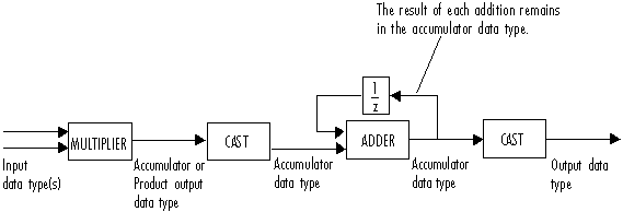
You can set the product output, accumulator, and output data types using the corresponding fixed-point properties of the object.

When the input is real, the output of the multiplier is in the product output data type. When the input is complex, the output of the multiplier is in the accumulator data type. For details on the complex multiplication performed, see Multiplication Data Types.

Note

When one or both of the inputs are signed fixed-point signals, all internal object data types are signed fixed point. The internal object data types are unsigned fixed point only when both inputs are unsigned fixed-point signals.

Documentation

dsp.Crosscorrelator

Description

Creation

Syntax

Description

Properties

Method — Domain for computing correlations 'Time Domain' (default) | 'Frequency Domain' | 'Fastest'

Fixed-Point Properties

FullPrecisionOverride — Full-precision override for fixed-point arithmetic true (default) | false

RoundingMethod — Rounding method for fixed-point operations 'Floor' (default) | 'Ceiling' | 'Convergent' | 'Nearest' | 'Round' | 'Simplest' | 'Zero'

Dependencies

OverflowAction — Overflow action for fixed-point operations 'Wrap' (default) | 'Saturate'

Dependencies

ProductDataType — Data type of product output 'Full precision' (default) | 'Custom' | 'Same as first input'

Dependencies

CustomProductDataType — Word and fraction lengths of product data type numerictype([],32,30) (default)

Dependencies

AccumulatorDataType — Data type of accumulation operation 'Full precision' (default) | 'Same as first input' | 'Same as product' | 'Custom'

Dependencies

CustomAccumulatorDataType — Word and fraction lengths of accumulator data type numerictype([],32,30) (default)

Dependencies

OutputDataType — Data type of object output 'Same as accumulator' (default) | 'Same as first input' | 'Same as product' | 'Custom'

Dependencies

CustomOutputDataType — Word and fraction lengths of output data type numerictype([],16,15) (default)

Dependencies

Usage

Syntax

Description

Input Arguments

u — First data input signal vector | matrix | N-D array

v — Second data input signal scalar | column vector | matrix

Output Arguments

y — Cross-correlated output vector | matrix | N-D array

Object Functions

Common to All System Objects

Examples

Compute Correlation Between Two Signals

Cross-Correlation of Input Noise and Delayed Version

More About

Cross-Correlation

Algorithms

Time-Domain Computation

Frequency-Domain Computation

Extended Capabilities

C/C++ Code Generation Generate C and C++ code using MATLAB® Coder™.

Fixed-Point Conversion Design and simulate fixed-point systems using Fixed-Point Designer™.

See Also

Objects

Blocks

DSP System Toolbox Documentation

Support

`Method` — Domain for computing correlations
`'Time Domain'` (default) | `'Frequency Domain'` | `'Fastest'`

`FullPrecisionOverride` — Full-precision override for fixed-point arithmetic
`true` (default) | `false`

`RoundingMethod` — Rounding method for fixed-point operations
`'Floor'` (default) | `'Ceiling'` | `'Convergent'` | `'Nearest'` | `'Round'` | `'Simplest'` | `'Zero'`

`OverflowAction` — Overflow action for fixed-point operations
`'Wrap'` (default) | `'Saturate'`

`ProductDataType` — Data type of product output
`'Full precision'` (default) | `'Custom'` | `'Same as first input'`

`CustomProductDataType` — Word and fraction lengths of product data type
`numerictype([],32,30)` (default)

`AccumulatorDataType` — Data type of accumulation operation
`'Full precision'` (default) | `'Same as first input'` | `'Same as product'` | `'Custom'`

`CustomAccumulatorDataType` — Word and fraction lengths of accumulator data type
`numerictype([],32,30)` (default)

`OutputDataType` — Data type of object output
`'Same as accumulator'` (default) | `'Same as first input'` | `'Same as product'` | `'Custom'`

`CustomOutputDataType` — Word and fraction lengths of output data type
`numerictype([],16,15)` (default)

`u` — First data input signal
vector | matrix | N-D array

`v` — Second data input signal
scalar | column vector | matrix

`y` — Cross-correlated output
vector | matrix | N-D array

C/C++ Code Generation
Generate C and C++ code using MATLAB® Coder™.

Fixed-Point Conversion
Design and simulate fixed-point systems using Fixed-Point Designer™.