Simscape HDL Workflow Advisor Tips and Guidelines
By using the Simscape HDL Workflow Advisor, you can generate an HDL implementation model.
You can generate HDL code for the implementation model and deploy the generated code onto FPGA
platforms. To open the Advisor, run the sschdladvisor
function. For example:
sschdladvisor('sschdlexHalfWaveRectifierExample')
The Simscape HDL Workflow Advisor consists of various tasks that convert your Simscape™ model to the HDL implementation model. When running various tasks in the Simscape HDL Workflow Advisor, you can follow certain tips and guidelines. You see these tips in the UI window of a particular task. For example, in the task that discretizes the equations to state-space parameters, the UI has a tip that suggests how to change the sample time. This section contains more information about each tip in the Simscape HDL Workflow Advisor UI.
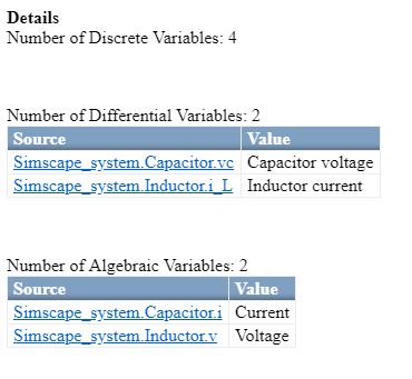
Estimating Resource Consumption Using Algebraic and Differential Variables
After you run the Check Switched Linear task, the task reports the
number of differential and algebraic variables for each Simscape network present in the model. For example, this figure illustrates that there
are two differential and two algebraic variables in the boost converter example model
sschdlexBoostConverterExample.
sschdladvisor('sschdlexHalfWaveRectifierExample')
Run the workflow to the Check Switched Linear task.
By viewing the number of algebraic and differential variables, you can determine how the
design consumes resources on the FPGA device. If Nd is the number of
differential variables and Na is the number of algebraic variables, the
resource usage on the target hardware varies according to the relation
Nd*(Nd+Na). Differential variables consume a quadratic amount of
multiplier resources on the target FPGA device. Algebraic variables consume a linear amount
of multiplier resources. You can use this information to determine how many multiplier
resources your Simscape design consumes on the FPGA device and whether your design is ready for
conversion to state-space representation.
Setting Simulation Stop Time for Extracting Equations
Change Simulation Stop Time
When you run the Extract Equations task, the Simscape HDL Workflow Advisor reports the simulation stop time. The simulation stop time corresponds to the amount of time that the Advisor takes to run simulation on your Simscape model. The stop time must not be significantly large such that the Advisor takes a long time to run this task. Use a stop time that is sufficient to reach the required number of modes for your model. To change the stop time, navigate to the Simscape model, and then specify the Stop Time.
Simulation Stop Time and Number of Modes
In the Extract Equations task, when you extract the differential algebraic equations, the Simscape HDL Workflow Advisor simulates the model to cover the nonlinear range of Simscape blocks. This task can take a long time depending on the number of switching elements in the Simscape model.
For a switched linear model, each switching element in the design has two modes. A
switched linear model with n switching elements has
2^n possible modes. For Simscape models with large number of switching elements, the number of modes can
become significantly large. For example, the Vienna rectifier has 21
switching elements, which translates to 2^21 possible modes. The
Simscape HDL Workflow Advisor can take a long time to simulate such a large model and
cover such a large number of modes. In addition, the HDL implementation model that you
generate for such a design can consume a large amount of resources or may not even fit on
the target FPGA device.
In most cases, while simulating the model, the Advisor does not have to reach the
entire 2^n modes. For example, consider this bridge rectifier model. To
open this model,
enter:
open_system('sschdlexBridgeRectifierExample')Inside the Simscape_system
Subsystem, you see the four diodes arranged in a bridge
configuration.

As each diode has two states, the Simscape design can have 2^4 = 16 possible states. In contrast,
the bridge rectifier has only three modes. The modes are:
Diodes
D1andD2areON,D3andD4areOFFDiodes
D1andD2areOFF,D3andD4areONDiodes
D1,D2,D3, andD4areOFF
This example shows that, based on the Simscape algorithm and the input to the design, you can set the simulation stop time to a minimum value that covers the number of modes to be reached.
Changing Sample Time for Discretizing Equations
Change Sample Time
When you run the Discretize Equations task, the Simscape HDL Workflow Advisor reports the discrete sample time. The discrete sample time corresponds to the sample time that the Advisor uses to discretize the differential algebraic equations to state-space parameters. To change the sample time, in your Simscape model, open the Block Parameters dialog box for the Solver Configuration block, and then specify the Sample time.
Sample Time and Discretizing Equations
In the Discretize Equations task, the Simscape HDL Workflow Advisor discretizes the differential algebraic equations into state-space parameters. You extract the differential algebraic equations by simulating the Simscape model in the previous task, Extract Equations. The Discretize Equations task runs much faster than the Extract Equations task because the Advisor only has to discretize the differential algebraic equations to state-space parameters.
The Discretize Equations task obtains the sample time information from the sample time that you specify for the Solver Configuration (Simscape) block in your model. The Advisor then discretizes the equations to state-space parameters based on this sample time information.
Using Number of Solver Iterations
What is Number of Solver Iterations?
In the Generate implementation model task, you can specify the Number of solver iterations. The number of solver iterations refer to the number of times the state-space model is executed per mode. The Simscape HDL Workflow Advisor generates the number of iterations that are required for executing the state-space model, automatically.
For each mode in the physical system, the switched linear workflow arrives at a state-space representation. The solver method is iterative and performs multiple computations to determine the correct mode for the next time step. After a certain number of iterations, the output value from the next time step becomes the same as the value from the previous time step. This consistency in the output value indicates the correct number of solver iterations.
By default, the Number of Solver iterations is
1 for linear models. For switched linear models, the Number
of solver iterations depends on the number of mode iterations that
Simscape uses during model simulation. This chosen value is optimal such that it
causes the model to converge and avoids exceeding the threshold value for real-time
deployment.
Using Fixed-Cost Runtime Consistency Iterations
On the Solver Configuration block, the Use fixed-cost runtime consistency iterations check box is cleared by default. If you select this check box, the Nonlinear iterations setting on the Solver Configuration block becomes the same as the Number of solver iterations setting in the Generate implementation model task.
By default, Nonlinear iterations is set to 2.
When you run the Generate implementation model task, the Advisor sets
the Number of solver iterations to 2 and this
setting cannot be modified. To modify the Number of solver
iterations, either:
Change Nonlinear iterations.
Clear Use fixed-cost runtime consistency iterations and then change the Number of solver iterations.
To learn more about the Use fixed-cost runtime consistency iterations setting, see Solver Configuration (Simscape). See also Solvers for Real-Time Simulation (Simscape).
Change Number of Solver Iterations
By default, you can change the number of solver iterations on this task. Increasing the number of solver iterations improves the numerical accuracy of generated HDL implementation model. To achieve higher sampling frequencies, reduce the number of solver iterations. Choose a value for number of solver iterations that trades off numerical accuracy and sampling frequency.
On the Solver Configuration block, if you specify the Use fixed-cost runtime consistency iterations setting, you cannot change the Number of solver iterations setting on this task. To change the number of solver iterations, on the Solver Configuration block, change the Nonlinear iterations parameter and rerun the Generate implementation model task.
Trading off Numerical Accuracy and Sampling Frequency
To verify whether the numeric results of the HDL implementation model matches the original Simscape model, select Generate validation logic for the implementation model. If the numeric results from the HDL implementation model do not match, you can increase the number of solver iterations. To learn more, see Increase Number of Solver Iterations.
Changing the number of solver iterations trades off numerical accuracy for sampling frequency. Increasing the number of solver iterations increases the sample time of the HDL implementation model which can reduce the sampling frequency. See Reducing Number of Solver Iterations.
Floating-Point Precision and Numerical Accuracy
Use the Floating-point precision setting to specify whether you
want the algorithm inside the HDL Subsystem in the generated
implementation model to use single or double data
types when performing the matrix computations.
| Floating-Point Precision | Description |
|---|---|
Double | Using double floating-point precision increases the
numerical accuracy of the generated model and the maximum achievable target
frequency. However, the area consumption and pipeline latency are also
increased. |
Single | This is the default setting for floating-point precision. |
Single coefficient, double computation | This mode offers a tradeoff between Single and
Double modes of floating-point precision. To save memory usage,
the coefficients that are stored in single. The matrix
computations are then performed in double for improved
accuracy. |
To learn more about the floating-point precision settings and tradeoffs, see Use Larger Floating-Point Precision.